When Donald Becker introduced the idea of a Beowulf cluster while working at NASA in the early 1990s, he forever changed the face of high-performance computing. Instead of institutions forking out millions of dollars for the latest supercomputer, they now could spend hundreds of thousands and get the same performance. In fact, a quick scan of the TOP500 project's list of the world's fastest supercomputers shows just how far-reaching the concept of computer clusters has become. The emergence of the Beowulf cluster—a computer cluster created from off-the-shelf components and that runs Linux—has had an unintended effect as well. It has captivated the imaginations of computer geeks everywhere, most notably, those who frequent the Slashdot news site.

Unfortunately, many people believe that Beowulfs don't lend themselves particularly well to everyday tasks. This does have a bit of truth to it. I, for one, wouldn't pay money for a version of Quake 4 that runs on a Beowulf! On one extreme, companies such as Pixar use these computer systems to render their latest films, and on the other, scientists around the world are using them this minute to do everything from simulations of nuclear reactions to the unraveling of the human genome. The good news is that high-performance computing doesn't have to be confined to academic institutions and Hollywood studios.

Before you make your application parallel, you should consider whether it really needs to be. Parallel applications normally are written because the data they process is too large for conventional PCs or the processes involved in the program require a large amount of time. Is a one-second increase in speed worth the effort of parallelizing your code and managing a Beowulf cluster? In many cases, it is not. However, as we'll see later in this article, in a few situations, parallelizing your code can be done with a minimum amount of effort and yield sizeable performance gains.

You can apply the same methods to tackle image processing, audio processing or any other task that is easily broken up into parts. As an example of how to do this for whatever task you have at hand, I consider applying an image filter to a rather large image of your friend and mine, Tux.

The first thing we need is a set of identical computers running Linux, connected to each other through high-speed Ethernet. Gigabit Ethernet is best. The speed of the network connection is one factor that can bring a fast cluster to a crawl. We also need a shared filesystem of some sort and some clustering software/libraries. Most clusters use NFS to share the hard drive, though more exotic filesystems exist, like IBM's General Parallel Filesystem (GPFS). For clustering software, there are a few available choices. The standard these days is the Message Passing Interface (MPI), but the Parallel Virtual Machine (PVM) libraries also should work just fine. MOSIX and openMOSIX have been getting a lot of attention lately, but they are used primarily for programs that are not specifically written to run on clusters, and they work by distributing threads in multithreaded programs to other nodes. This article assumes you have MPI installed, though the process for parallelizing an algorithm with PVM is exactly the same. If you have never installed MPI, Stan Blank and Roman Zaritski have both written nice articles on how to set up an MPI-based cluster on the Linux Journal Web site (see the on-line Resources).

At the beginning of each MPI program are a few calls to subroutines that initialize communication between the computers and figure out what “rank” each node is. The rank of a node is a number that identifies it uniquely to the other computers, and it varies from 0 to one less than the total cluster size. Node 0 typically is called the master node and is the controller for the process. After the program is finished, you need to make one additional call to finish up the process before exiting. Here's how it's done:

#include <mpi.h>
#include <stdlib.h>

int main (void) {

           int myRank, clusterSize;
           int imgHeight, lowerBoundY, upperBoundY,
                boxSize;

          // Initialize MPI
         MPI_Init((void *) 0, (void *) 0);

         // Get which node number we are.
         MPI_Comm_rank(MPI_COMM_WORLD, &myRank);

         // Get how many total nodes there are.
         MPI_Comm_size(MPI_COMM_WORLD, &clusterSize);

        // boxSize - the amount of the image each node
        //                  will process
        boxSize = imgHeight / clusterSize;

         // lowerBoundY - where each node starts processing.
         lowerBoundY = myRank*boxSize;

        // upperBoundY - where each node stops processing.
        upperBoundY = lowerBoundY + boxSize;

        // Body of program goes here

        // Clean-up and exit:
        MPI_Finalize(MPI_COMM_WORLD);
        return 0;
}

This code runs independently on each machine that is part of the process, so the values for lowerBoundY and upperBoundY will vary on each machine. These will be used in the next section.

Figure 1. The process of breaking up a problem into smaller chunks is called domain decomposition, and it usually is done as shown here.

Applying a filter to an image can take minutes or even hours to complete, depending on the complexity of the filter, the size of the image and the speed of the computer. To fix these problems, we need to get smaller chunks of the image to several computers to help speed up the task. Figure 1 shows common ways of doing this—we'll cut our image into strips. If we have one large image file, we can do this in C/C++, like this:

FILE *imageFile = fopen("image_in.ppm", "rb");

// Safety check.
if (imageFile != NULL) {

   // Read in the header.
   fread(imageHeader, sizeof(char),
                    HEADER_LENGTH, imageFile);

   // fseek puts us at the point in the image
   // that this node will process.
   fseek(imageFile, lowerBoundY*WIDTH*3,
             SEEK_SET);

   // Here is where we read in the colors:
   // i is the current row in the image.
   // j is the current column in the image.
   // k is the color, 0 for red, 1 for blue,
   //    and 2 for green.
   for (i=0; i<boxSize+1; i++) {
      for (j=0; j<WIDTH; j++) {
         for(k=0; k<3; k++) {
           fread(&byte, 1, 1, imageFile);
            pixelIndex = i*WIDTH+j+k;
            origImage[pixelIndex] = byte;
         }
      }
   }
}
fclose(imageFile);

Now that we have each node storing a piece of the image for processing, we need to apply the filter to the image. The GIMP Documentation Team has done a good job of describing how to do this using a convolution matrix in the GIMP Documentation. Many image effects—such as sharpen, blur, Gaussian blur, edge detect and edge enhance—have unique matrices that provide the desired effect. The convolution matrix works by studying each pixel of an image and changing its value based on the values of neighboring pixels. We consider the edge detect matrix in this article, shown in Figure 2.

Figure 2. This matrix represents the edge detect filter. The red square represents the pixel to be considered, and the other numbers represent the neighboring pixels.

When we apply this filter to the image, we multiply each pixel by –4 and add the values of the pixels above, below and to the left and right to that. This becomes the new value of the pixel. Because there are zeros in the corners of the matrix, we can simplify our program and get better performance by skipping those calculations. Below I've shown how this is done in practice. In Figure 3, I show what the filter does to our image of Tux.

for (i=0; i<boxSize; i++) {
   for (j=0; j<WIDTH; j++) {
      if (i>0 && i<(HEIGHT-1) &&
          j>0 && j<(WIDTH-1)){

        // Now we apply the filter matrix

        // First to the current pixel.
        pixelIndex = i*WIDTH + j;
        r = origImage[pixelIndex];
        g = origImage[pixelIndex+1];
        b = origImage[pixelIndex+2];
        filter_r = -4*r;
        filter_g = -4*g;
        filter_b = -4*b;

        // Next to the left neighbor.
        pixelIndex = i*WIDTH + j - 1;
        r = origImage[pixelIndex];
        g = origImage[pixelIndex+1];
        b = origImage[pixelIndex+2];
        filter_r += 1*r;
        filter_g += 1*g;
        filter_b += 1*b;

        // Next to the right neighbor.
        pixelIndex = i*WIDTH + j + 1;
        r = origImage[pixelIndex];
        g = origImage[pixelIndex+1];
        b = origImage[pixelIndex+2];
        filter_r += 1*r;
        filter_g += 1*g;
        filter_b += 1*b;

        // The neighbor above.
        pixelIndex = (i-1)*WIDTH + j;
        r = origImage[pixelIndex];
        g = origImage[pixelIndex+1];
        b = origImage[pixelIndex+2];
        filter_r += 1*r;
        filter_g += 1*g;
        filter_b += 1*b;

        // The neighbor below.
        pixelIndex = (i+1)*WIDTH + j;
        r = origImage[pixelIndex];
        g = origImage[pixelIndex+1];
        b = origImage[pixelIndex+2];
        filter_r += 1*r;
        filter_g += 1*g;
        filter_b += 1*b;
      }

      // Record the new pixel.
      pixelIndex = i*WIDTH + j;
      filterImage[pixelIndex]   = filter_r;
      filterImage[pixelIndex+1] = filter_g;
      filterImage[pixelIndex+2] = filter_b;
   }
}

We can mimic the readImage() subroutine to create a writeImage() subroutine to write the image to disk in chunks.

Figure 3. On the left is our original image of Tux, and on the right is the image after we apply the edge detect filter.

Both of the popular MPI distributions—LAM and MPICH—include wrapper scripts to allow users to compile their programs easily with the required MPI libraries. These wrapper scripts allow you to pass parameters to GCC like you always do:

Use mpirun to execute your newly compiled program. For example, I compiled my code with the command mpicc -O3 -o parallel parallel.c and then executed it with mpirun n0 ./parallel. The n0 signifies that the program is to run on node 0 only. To run it on additional nodes, you can specify a range like n0-7 (for eight processors) or use mpirun C to signify that the program is to run on all available nodes.

So, with only a few simple MPI calls, we have parallelized our image filter algorithm very easily, but did we gain any performance? There are a few ways that we can gain performance. The first is in terms of speed, and the second is in terms of how much work we can do. For example, on a single computer, a 16,000 x 16,000 pixel image would require an array of 768,000,000 elements! This is just too much for many computers—GCC complained to me that the array was simply too big! By breaking the image down as we did above, we can ease memory requirements for our application.

I tested the code above on a 16-node Beowulf cluster running Fedora Core 1. Each node had 1.0GB of RAM, a 3.06GHz Pentium 4 processor and was connected to the other nodes through Gigabit Ethernet. The nodes also shared a common filesystem through NFS. Figure 4 shows the amount of time required to read in the image, process it and write it back to disk.

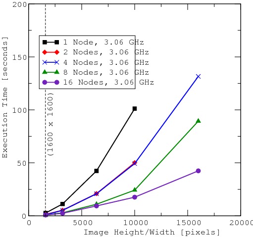
Figure 4. Shown here are the times that the program took for various image sizes and various cluster sizes. Image sizes ranged from 1,600 x 1,600 pixels to 16,000 x 16,000 pixels. A minimum of four nodes was required for the largest image.

From Figure 4, we can see that parallelizing this image filter sped things up for even moderately sized images, but the real performance gains happened for the largest images. Additionally, for images of more than 10,000 x 10,000 pixels, at least four nodes were required due to memory constraints. This figure also shows where it is a good idea to parallelize the code and where it was not. In particular, there was hardly any difference in the program's performance from 1,600 x 1,600 pixel images to about 3,200 x 3,200 pixel images. In this region, the images are so small that there is also no benefit in parallelizing the code from a memory standpoint, either.

To put some numbers to the performance of our image-processing program, one 3.06GHz machine takes about 50 seconds to read, process and write a 6,400 x 6,400 image to disk, whereas 16 nodes working together perform this task in about ten seconds. Even at 16,000 x 16,000 pixels, 16 nodes working together can process an image faster than one machine processing an image 6.25 times smaller.

This article demonstrates only one possible way to take advantage of the high performance of Beowulf clusters, but the same concepts are used in virtually all parallel programs. Typically, each node reads in a fraction of the data, performs some operation on it, and either sends it back to the master node or writes it out to disk. Here are four examples of areas that I think are prime candidates for parallelization:

I hope that this article has shown how parallel programming is for everybody. I've listed a few examples of what I believe to be good areas to apply the concepts presented here, but I'm sure there are many others.

There are a few keys to ensuring that you successfully parallelize whatever task you are working on. The first is to keep network communication between computers to a minimum. Sending data between nodes generally takes a relatively large amount of time compared to what happens on single nodes. In the example above, there was no communication between nodes. Some tasks may require it, however. Second, if you are reading your data from disk, read only what each node needs. This will help you keep memory usage to a bare minimum. Finally, be careful when performing tasks that require the nodes to be synchronized with each other, because the processes will not be synchronized by default. Some machines will run slightly faster than others. In the sidebar, I have included some common MPI subroutines that you can utilize, including one that will help you synchronize the nodes.

In the future, I expect computer clusters to play an even more important role in our everyday lives. I hope that this article has convinced you that it is quite easy to develop applications for these machines, and that the performance gains they demonstrate are substantial enough to use them in a variety of tasks. I would also like to thank Dr Mohamed Laradji of The University of Memphis Department of Physics for allowing me to run these applications on his group's Beowulf cluster.

Resources for this article: /article/9135.