Quantum GIS: the Open-Source Geographic Information System
If you've ever zoomed around the globe with Google Earth, you know how much fun it can be to work with geospatial data. When I need a diversion, I often fire up Google Earth and float above the skyscrapers of Manhattan or revisit former stomping grounds.
For a deeper level of control with geospatial information—where you're the chef who concocts the whole stew—dive into a geographic information system, or GIS. A GIS lets you control all the elements that go into the geophysical world you want to explore. Stripping GIS down to its essentials, you could call it computer-based mapmaking. However, because a GIS is powered by a database, the opportunities for advanced analysis are light-years beyond anything you could do with a paper-based map. A GIS not only will make you feel like you have the world in your hands—look out for that “I'm playing God” feeling—but you also probably will do something extremely useful with it for your work or private life.
This article introduces a sample project with Quantum GIS (QGIS), one of the most advanced and powerful open-source GIS packages for the desktop. Although QGIS has some excellent documentation, new users might find the terminology a bit stilted and missing some information. The authors of the documentation assume you already are familiar with GIS and that you're coming to QGIS from a proprietary alternative, such as the popular ArcGIS from ESRI. I, on the other hand, assume you've never used a GIS before.
To illustrate some basic functions of a desktop GIS, I use QGIS to make preparations for a fantasy of mine, which is to create an ecologically friendly real-estate development. In this exercise, I locate a parcel of agricultural land in Washtenaw County, Michigan, near Ann Arbor, where I can restore a former wetland and build a cluster of homes nearby. I chose Ann Arbor due to its proximity to drained wetlands in rural areas, as well as local demand for homes in areas with lots of wildlife.
To accomplish this task, I explore how to load QGIS on your system; find the geospatial data for the task; load that data into QGIS; and view, set up and analyze that data to do the job at hand. Along the way, I introduce key concepts and important terms.
QGIS has a useful, comprehensive Web site with plenty of resources to get you started. Beyond the free application download, you'll find a wiki, help forums and loads of documentation. QGIS has versions for Mac OS X, Windows and several variants for Linux users: source, Debian, Ubuntu Gutsy and OpenSUSE. Given that repositories are provided, installation should be easy and straightforward. All you need to do is add the requisite repository to your favorite package manager. If you must install from source, there are plenty of on-line guides explaining the process. See Figure 1 for a look at QGIS's GUI.
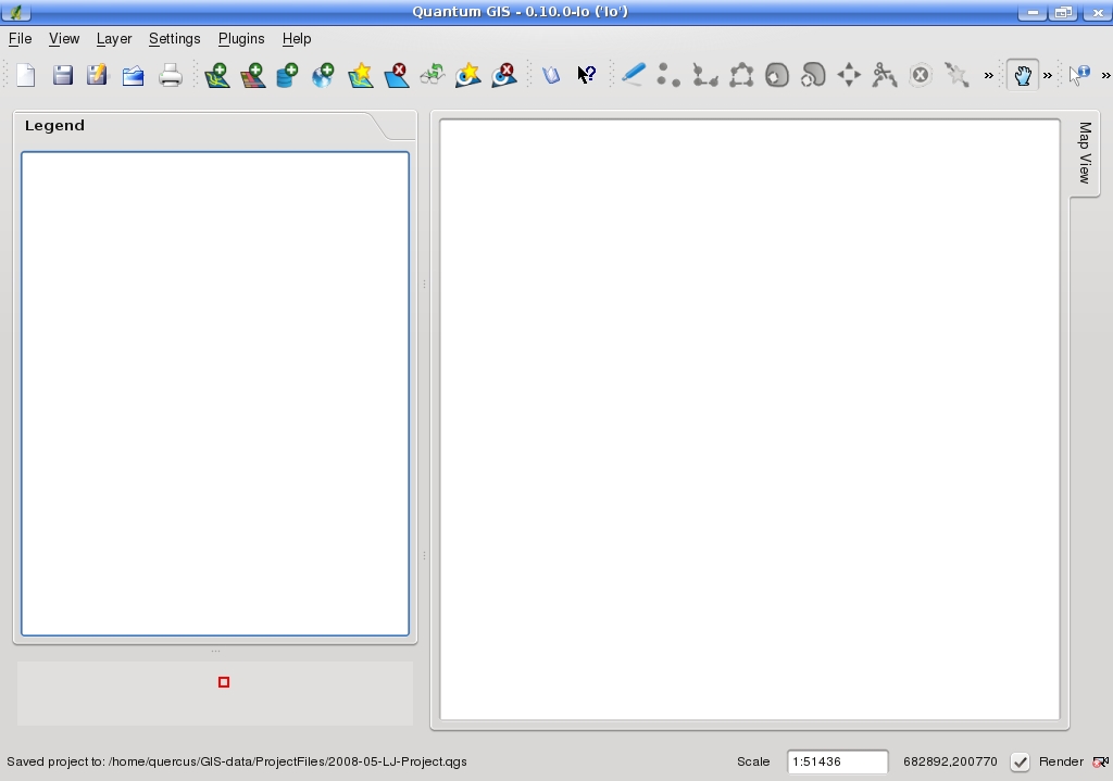
Figure 1. The application QGIS 0.10 offers a clean, intuitive user interface.
GIS is a complex application requiring knowledge about data formats, how a GIS functions and general cartography. Let's rip through a quick, need-to-know primer on GIS.
As mentioned previously, using a GIS is essentially mapping on a computer. To do this mapping, you need to find data related to geography, typically called geospatial data. This geospatial data that we will introduce into QGIS consists of two elements, namely spatial features and attribute data. Examples of spatial features might include streets, rivers or land cover—any feature you might find on a map. Meanwhile, attribute data describes the characteristics of the spatial features and is stored in a database within the GIS. For example, most of those streets have names and lengths; the land-cover types have names and areas associated with them. In the case of land cover, a GIS might store attribute-related categories, such as high-density urban, low-density urban, cropland, forest and so on, which you then could query easily.
Your paper road map would think you were completely mad if you commanded it to “just show me the rivers and mountains, please” or “flip the county boundaries on and off”. On the other hand, because a GIS portrays data in similar groupings of geographic elements, called layers, your computer will execute your command and not label you loopy. Some examples of layers are countries, cities, rivers and oceans. A GIS allows you to control which layers are displayed on your screen at any time.
Layers can consist of two types, namely features and surfaces. In our above list, the layers with countries, cities, rivers and specific buildings are feature-based; oceans are one single, continuous expanse and, thus, are a surface.
The hefty challenge for a GIS is to portray our lovely yet complex world accurately yet rapidly—and without the need for a cluster! There are two tricks, or methods, a GIS uses to create a digital representation of Earth's features on your desktop.
The first method is using vector data (the type used later in this article). As complicated as the world can be, a GIS can represent any geographical object using three geometric elements—namely points, lines and polygons. Small stuff like community centers and traffic lights can be portrayed as points. Features such as rivers and pipelines are really just glorified lines, so they can be shown as such. Finally, nearly everything else, such as a state park, though it might be oddly shaped, is finite and contained in boundaries, making it a polygon at the end of the day. Broadly speaking, the vector format is analogous to traditional maps, where the world is abstracted with symbology, and precision is very important.
The second method is raster data. Raster data is used to portray Earth's characteristics that have no shape visually, including measurements like ocean depth, forest-cover type, elevation and annual rainfall. Some image types you will encounter include GeoTIFFs, Erdas Imagine Images, GRASS AIGs and USGS Digital Elevation Models. Some common examples of raster-based imagery are satellite images and aerial photos. In these two types of raster imagery, the value of each cell is a measurement of light that is reflected off the Earth's surface. Particular ranges of these values can signify specific land-cover or vegetation types.
As you splash around in the world of GIS, you also will encounter a plethora of vector-based spatial file formats. If you have ever used the application ArcGIS from ESRI, you probably are familiar with geodatabases and coverages, two of the most common spatial file formats in proprietary GIS. Of these two more-advanced spatial data formats, only coverages are usable in QGIS, but not geodatabases. In addition, in QGIS, we can utilize ESRI shapefiles, which are plentiful in on-line data repositories and a sort of standard, as they have been around a long time. In fact, shapefiles are the standard format for ESRI's ArcView, which is the company's previous generation of GIS applications. Essentially, a shapefile is a set of files with vector-based location and attribute data, which can be represented in a GIS application.
QGIS also supports some other file formats, such as MapInfo and PostGIS. PostGIS is especially interesting, as it is an open-source spatial database technology. PostGIS “spatially enables” the PostgreSQL server, allowing it to be used as a back-end spatial database for GIS and—for those who are familiar with GIS technologies—as such, is similar to ESRI's SDE or Oracle's Spatial extension.
Two other important concepts critical to any cartographic endeavor are map projections and coordinate systems.
Remember the big, flat world map you had in your fourth-grade classroom? The one with Greenland bigger than Africa? That map is an ideal illustration of what happens when you depict a round object such as the earth onto a flat map. Converting a 3-D globe onto a 2-D map is called a map projection.
In a GIS, you need to consider the projection, because any map you view or create is essentially flat like a paper map. Thus, the same concept applies to both situations.
Just as important as the map projection is the coordinate system. A coordinate system is the Cartesian system of x and y axes that a GIS uses to define locations on a map. This is opposed to the latitude and longitude system that defines location on a sphere.
In larger projects, knowledge of projections and coordinate systems is very important, and if a mismatch exists among different parts of a project, life can get frustrating quickly. Fortunately, this project is simple enough to avoid much concern, as I am working at the county level and all my shapefiles come from the same data source. However, when working with larger areas and multiple data sources, it is important to be familiar with these concepts and standardize your projection and coordinate system project-wide.
At this point, we have enough GIS theory to understand what we're doing and start the real-estate planning project. At this stage, I track down the requisite data.
This project involves finding a parcel of land in Washtenaw County, Michigan, where I can build a cluster of homes in a natural setting. I am looking for a suitable land parcel that was once a wetland but today is agricultural and suitable for conversion back to a wetland. The ideal site will be close to a river or lake, have good road access and be as close to the city of Ann Arbor as possible.
When you embark on a GIS-based project, it's wise to specify all of the elements you need, because in general, each will likely be one of the layers you must acquire. Thus, for this project, we need layers that depict, respectively, land use, areas with potential for wetland restoration, roads and hydrography (rivers and lakes). In general, the most common format for each layer will be in the form of a shapefile, which QGIS can handle without a hitch.
So where can I obtain these shapefiles? Fortunately, a plethora of excellent repositories of free, downloadable geospatial data exist. An excellent example is the public Michigan Geographic Data Library (MGDL), which offers a vast collection of vector- and raster-based data at the watershed, county and state levels. Just some of the datasets available include those I am looking for, as well as aerial photos of the entire state, federal census information, geology, soil types, public land ownership and topography. In the MGDL, the default format for vector-based data is the shapefile.
From the MGDL, I can download the following datasets at the county extent:
Michigan Geographic Framework Hydrography (lakes and rivers).
1992 National Land Cover Dataset.
Michigan Geographic Framework Transportation (roads).
Potential Wetland Restoration.
Loading shapefiles into QGIS is done by clicking the toolbar icon labeled Add vector layer, which looks like a plus sign hovering over a map; it opens a standard open file dialog. By preselecting ESRI shapefile (suffix .shp) from Files of Type, I can be sure I'm opening the right file, which is useful, because a shapefile is actually a bundle of files. As I load each shapefile, it shows up under its original name on the left under the Legend window, which acts as a sort of table of contents.
After unpacking the datasets, I load these five shapefiles in this order: allroads_161v7b.shp (roads), hydro_161v7b.shp (rivers), hydropoly_161v7b.shp (lakes), Washtenaw_Potential_Restoration_Area.shp (the name says it all) and Washtenaw_nlcd_1992.shp (land use).
Unfortunately, upon loading the shapefiles, the sum total map that's displayed on the right in the Map View window looks like a big rectangle covered with random black and green blobs and no lines. Where are the roads, lakes and rivers I loaded? One reason for the odd display and missing elements is that the layers I added first are buried under the county-wide land-use layer, which sits on top of everything else. I can begin to solve this problem by dragging the land-use layer down to the bottom of the Legend and tinkering with the other layers so they all are visible.
The other reason for the strange-looking map is that QGIS defaults to display one color for every characteristic in the shapefile. For the road layer, defaulting to one color is fine, because it is simply a collection of lines. However, layers with thousands of polygons are more complicated. All of the many land-use types default to the same color, thus creating no differentiation among them. I must give each land-use type its own unique color manually. To do so, I first right-click on the land-use entry in the legend and select Properties from the menu. On the Symbology tab, I change the drop-down menu next to Legend type from the default value of Single Symbol to Unique Value. Using the drop-down menu in Classification Field, I can select which field in the database to classify. In my case, I classify a field called GRIDCODE, which contains the code that designates the land-use code for each polygon in the layer.
How do I know which database field I should classify, as well as the meaning of each classification? To find out, I sometimes need to leave the Layer Properties menu and examine the attribute table, a display of the database containing the attribute data for the layer. For example, I can examine the attribute table of the land-use layer by right-clicking on the title in the Legend (on the main GUI) and selecting the command Open attribute table. An example of an attribute table is shown in Figure 2. The land-use attribute layer contains a field ID to designate each polygon, as well as the field GRIDCODE to classify each one. Oftentimes the attribute table also contains a field with the label for each classification. Although such a field is missing from the land-use attribute table, a separate file with classifications is found in a text file included in the downloaded dataset.
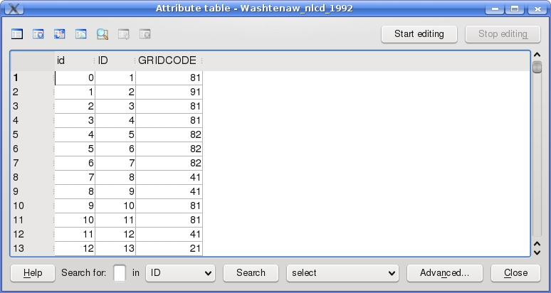
Figure 2. The attribute table displays the data contained in a particular layer, for example, a shapefile.
After consulting the attribute table and the file containing classifications, I am ready to continue with the classification of the field GRIDCODE back in the Layer Properties menu. Pressing the Classify button populates the window below with the unique classification codes found in the layer. I can label each classification as I wish using the "Label" field, and I can give each classification its own color with the Fill color option.
After finishing the classification, I also want to do some more housekeeping to make the Legend and Map View more useful, such as making the colors of the other layers more intuitive (for example, blue lakes) and thickening the lines designating the roads and rivers. I can carry these out also with the Layer Properties dialog (right-click on layer name→Properties). A right-click on the layer name also gives me the option to change the layer name displayed in the Legend.
Post-housekeeping, the Map View in QGIS finally takes shape. I finally can recognize features such as roads and rivers, and now that the land-use types are differentiated, I easily can tell which areas are urban, agricultural, forested and so on. Figure 3 shows the end result.
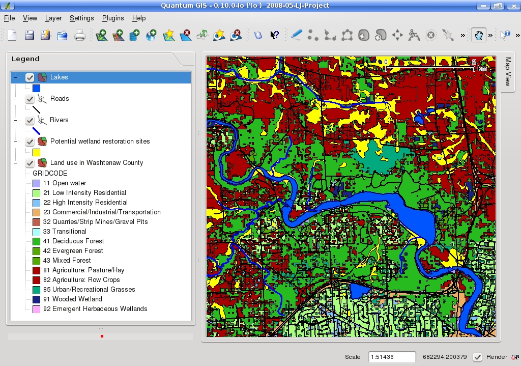
Figure 3. After modifying the properties of each layer and changing the layer names in the Legend, the Map View is readable and ready for analysis.
To simplify visual analysis on my map, I also applied the same color to similar land-use categories. For instance, I applied the same color to two different agricultural categories as well as three different forest-related ones. For this application, I am interested to know only whether the land use is agricultural or forested, not the specific type of each. Fewer colors makes my map less busy.
Although QGIS contains several essential tools, I briefly discuss only three here: the Pan, Zoom and Identify Features tools.
The most essential tool for navigating around a layer is the Pan tool, the toolbar icon in the shape of a hand. If I click on that tool, I quickly can drag my map around the Map View window.
However, if I want to change the level of detail in the Map View, I must switch to the Zoom tool. Although the Zoom tool is intuitive in function, beware, for it is disappointingly unintuitive in practice for three reasons. First, the Zoom tool resides in the View menu and is not available as a toolbar option. Second, the Zoom In and Zoom Out functions work only using the wheel of a mouse. Because I work on a laptop, I had to acquire a USB mouse just to have zooming capabilities. Third, unlike with most GIS and graphics applications, QGIS does not simply allow one to draw a box around the desired zoom-to area.
Meanwhile, the Identify Features tool is more straightforward and less cumbersome. To activate the tool, I simply press the toolbar icon designated by a mouse arrow next to the letter i in a blue circle. Then, I can navigate to any feature in the Map View window and essentially call up that feature's characteristics—that is, its entry in the attribute table. In order to select the appropriate feature, however, I must select the correct layer in the Legend. For example, if I am searching for information about a lake, I can't be on the Roads layer—the Lakes layer must be selected. Figure 4 shows how I clicked on a large lake and learned its size, elevation and name, Ford Lake.
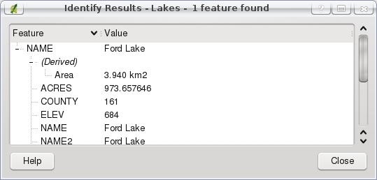
Figure 4. The Identify Features tool gives you detailed information on a particular feature. Be sure you've chosen the right layer in the Legend.
Now that I've covered the basics of GIS, found the requisite shapefiles, loaded those files into QGIS and explored basic navigation, it's time to find and record locations for my housing project. To find ideal sites where I can restore a wetland on agricultural land close to Ann Arbor, I pan and zoom around my map and toggle layers on and off.
After searching for a time, I decide to save some sites for later reference. The best way to do this is to create my own layer (shapefile). To do this, I click on the New Vector Layer icon in the toolbar, and because all I need are specific locations, I opt for a point-based shapefile. At the same time, I must build an attribute table, which I do by clicking on the Add Attribute button. I need only one string-based field, which I label Locations.
Now that I have my own shapefile, as long as that layer is selected in the Legend, I can add my own points to it by selecting the Toggle Editing tool. Once the tool is selected, the button right next door on the toolbar, the Capture Point tool, is activated, and I can create points anywhere I choose. I create a point for each potential building site I find and add a label to each, as prompted by QGIS. I press the Toggle Editing icon once again to leave edit mode and return to normal browse mode.
Thus far, QGIS has been useful in giving me a broad perspective on natural and man-made features, as well as land-use characteristics. This is much more than what nearly every paper map or Google Earth will give me. Still, QGIS can't do everything. Unfortunately, I probably can't acquire a shapefile with current land-ownership status. Therefore, I must utilize other resources, such as the County Clerk, in order to discover who owns which parcels. Clearly my work has only just begun.
The free and open-source QGIS turns out to be an appropriate tool for projects involving land use, such as my search for a site to restore a wetland and build an eco-friendly housing development. In this project, I was able to locate the geospatial data I needed from a free geospatial data repository, load it into QGIS, tailor the data to my liking and designate a plethora of potential building sites. Besides land-use projects, you also can delve into demographic data, satellite and aerial-photo imagery, other natural and man-made features and more. Although cramming on GIS concepts and conventions was required, working with QGIS and other GIS applications, although a bit challenging at first, is extremely useful, rewarding and fun.
Resources
QGIS Home Page: www.qgis.org
QGIS Download Repositories: download.qgis.org/downloads.rhtml
OSGEO Home Page: www.osgeo.org
Michigan Geographic Data Library: www.mcgi.state.mi.us/mgdl
James Gray is Linux Journal Products Editor and a graduate student in environmental science and management at Michigan State University. A Linux enthusiast since the mid-1990s, he currently resides in Lansing, Michigan, with his wife and cats.