
Modeling the Brain with NCS and Brainlab
Computer scientists have been studying artificial neural networks (ANNs) since the 1950s. Although ANNs were inspired by real biological networks like those in your brain, typical ANNs do not model a number of aspects of biology that may turn out to be important. Real neurons, for example, communicate by sending out little spikes of voltage called action potentials (APs). ANNs, however, do not model the timing of these individual APs. Instead, ANNs typically assume that APs are repetitive, and they model only the rate of that repetition. For a while, most researchers believed that modeling the spike rate was enough to capture the interesting behavior of the network. But what if some of the computational power of a biological neural network was derived from the precise timing of the individual APs? Regular ANNs could never model such a possibility.
In 1999, the thought that ANNs were overlooking the reality of individual APs convinced Phil Goodman at the University of Nevada, Reno, to change his focus from ANNs to more realistic spiking neural network models. He started by looking for a program that would allow him to conduct experiments on large networks of spiking neurons. At the time, a couple of excellent open-source research software packages existed that were capable of simulating a few spiking neurons realistically; GENESIS and NEURON were two of the most popular. But these programs were not designed to work with the networks of thousands of spiking neurons that he was envisioning. Goodman believed that with low-cost Linux clustering technology, it should be possible to construct a parallel program that was realistic enough to model the spiking and cellular membrane channel behavior of neurons, while also being efficient enough to allow the construction of large networks of these neurons for study. Goodman launched the NeoCortical Simulator (NCS) Project to create such a program. Starting with a prototype program that Goodman wrote in the proprietary MATLAB environment, a student working with computer science professor Sushil Louis wrote the first parallel version of NCS in C using the MPI parallel library package.
When I joined the research group in 2002, NCS already was undergoing a major rewrite by another student, James Frye, who was working with CS professor Frederick C. Harris, Jr. This time, the goal was to take the system from prototype to streamlined and reliable production software system. I helped with this effort, implementing a number of optimizations that greatly improved performance.
I also set up the first version control for the NCS source code, using the then-new open-source Subversion system. At the time, Subversion still was an alpha project. Nevertheless, I was sold on several features of the system, including the automatic bundling of an entire set of files into a single release. After working with Subversion a bit, the old workhorse CVS seemed cumbersome in comparison. Subversion was evolving quickly then. More than once after a system software upgrade, though, I had to spend hours trying to rebuild a Subversion executable with a certain combination of component library versions that would restore access to our version history. The Subversion user mailing list always was helpful during these recovery efforts. Eager to take advantage of the new features, I willingly paid the price for choosing alpha software. Fortunately, that trade-off is no longer necessary. Subversion now is stable and flexible, and I would not hesitate to choose it for any new project.
As the NCS software matured, our cluster expanded, thanks to several grants from the US Office of Naval Research. The initial Beowulf cluster of 30 dual-processor Pentium III machines grew with the addition of 34 dual-processor Pentium 4s. It grew again recently with the addition of 40 dual-processor Opterons. Linux has been the OS for the cluster from the start, running the Rocks cluster Linux release. The compute nodes are equipped with a full 4GB of system memory to hold the large number of synapse structures in the brain models. Memory capacity was a major motivation for moving to the 64-bit Opterons. Administrative network traffic moves on a 100MB and, later, 1GB Ethernet connection, while a specialized low-latency Myrinet network efficiently passes the millions of AP spike messages that occur in a typical neural network simulation.
With NCS now capable of simulating networks of thousands of spiking neurons and many millions of synapses, students began to use it for actual research. NCS could be quite hard to use effectively in practice, however, as I discovered when I began my own first large-scale simulation experiments. Much of the difficulty in using NCS stemmed from the fact that NCS takes a plain-text file as input. This input file defines the characteristics of the neural network, including neuron and dendrite compartments, synapses, ion channels and more. For a large neural network model, this text file often grows to thousands or even hundreds of thousands of lines.
Although this plain-text file approach allows a great deal of flexibility in model definition, it quickly becomes apparent to anyone doing serious work with NCS that it is not practical to create network models by directly editing the input file in a text editor. If the model contains more than a handful of neural structures, hand-editing is tedious and prone to error. So every student eventually ends up implementing some sort of special purpose macro processor to help construct the input file by repeatedly emitting text chunks with variable substitutions based on a loop or other control structure. Several of these preprocessors were built in the proprietary MATLAB language, because MATLAB also is useful for the post-simulation data analysis and is a popular tool in our lab. Each of these macro processors was implemented hurriedly with one specific network model in mind. No solution was general enough to be used by the next student, therefore, causing a great deal of redundant effort.
I searched for a more general solution, both for my own work and to prevent future students from facing these familiar hurdles as they started to use NCS for large experiments. No templated preprocessing approach seemed up to the task. After a bit of experimentation, I concluded that the best way of specifying a brain model was directly as a program—not as a templated text file that would be parsed by a program, but actually as a program itself.
To understand the problem, consider that our brain models often contain hundreds or thousands of structures called cortical columns, each made up of a hundred or more neurons. These columns have complex, often variable internal structures, and these columns themselves are interconnected by synapses in complex ways. We might want to adjust the patterns of some or all of these connections from run to run. For example, we might want to connect a column to all neighbor columns that lie within a certain distance range, with a certain probability that is a function of the distance. Even this relatively simple connection pattern can't be expressed conveniently in the NCS input file, which permits only a plain list of objects and connections.
But, by storing the brain model itself as a small script that constructs the connections, we could have a model in only a few lines of code instead of thousands of lines of text. This code easily could be modified later for variations of the experiment. All the powerful looping and control constructs, math capabilities and even object orientation of the scripting language could be available directly to the brain modeler. Behind the scenes, the script automatically could convert the script representation of the model into the NCS text input file for actual simulation. No brain modeler ever would be bound by a restrictive parsed template structure again. I gave the generalized script-based modeling environment that I planned to develop the name Brainlab and set to work picking a suitable scripting language for the project.
My first thought for a scripting language was MATLAB, given its prominence in our lab. But repeated licensing server failures during critical periods had soured me on MATLAB. I considered Octave, an excellent open-source MATLAB work-alike that employed the same powerful vector processing approach. I generally liked what I saw and even ported a few MATLAB applications to work in Octave in a pinch. I was pleased to find that the conversions were relatively painless, complicated only by MATLAB's loose language specification. But I found Octave's syntax awkward, which was no surprise because it largely was inherited from MATLAB. My previous Tcl/Tk experiences had been positive, but there didn't seem to be much of a scientific community using it. I had done a few projects in Perl over the years, but I found it hard to read and easy to forget.
Then I started working with Python on a few small projects. Python's clean syntax, powerful and well-designed object-oriented capabilities and large user community with extensive libraries and scientific toolkits made it a joy to use. Reading Python code was so easy and natural that I could leave a project for a few months and pick it up again, with barely any delay figuring out where I was when I left off. So I created the first version of Brainlab using Python.
In Brainlab, a brain model starts as a Python object of the class BRAIN:
from brainlab import *
brain=BRAIN()
This brain object initially contains a default library of cell types, synapse types, ion channel types and other types of objects used to build brain models. For example, the built-in ion channel types are stored in a field in the BRAIN class named chantypes. This field actually is a Python dictionary indexed by the name of the channel. It can be viewed simply by printing out the corresponding Python dictionary:
print brain.chantypes
A new channel type named ahp-3, based on the standard type named ahp-2, could be created, modified and then viewed like this:
nc=brain.Copy(brain.chantypes, 'ahp-2', 'ahp-3')
nc.parms['STRENGTH']="0.4 0.04"
print brain.chantypes['ahp-3']
To build a real network, the brain must contain some instances of these structures and not only type profiles. In NCS, every cell belongs to a structure called a cortical column. We can create an instance of a simple column and add it to our brain object like this:
c1=brain.Standard1CellColumn()
brain.AddColumn(c1)
This column object comes with a set of default ion channel instances and other structures that we easily can adjust if necessary. Most often we have a group of columns that we want to create and interconnect. The following example creates a two-dimensional grid of columns in a loop and then connects the columns randomly:
cols={}
size=10
# create the columns and store them in cols{}
for i in range(size):
    for j in range(size):
        c=brain.Standard1CellColumn()
        brain.AddColumn(c)
        cols[i,j]=c
# now connect each column to another random column
# (using a default synapse)
for i in range(size):
    for j in range(size):
        ti=randint(0, size-1)
        tj=randint(0, size-1)
        fc=cols[i,j]; tc=cols[ti,tj]
        brain.AddConnect(fc, tc)
Our brain won't do much unless it gets some stimulus. Therefore, we can define a set of randomly spaced stimulus spikes in a Python list and apply it to the first row of our column grid like this:
t=0.0
stim=[]
for s in range(20):
    t+=random()*10.0
    stims.append(t)
for i in range(size):
    brain.AddStim(stim, cols[i,0])
So far, our brain model exists only as a Python object. In order to run it in an NCS simulation, we have to convert it to the text input file that NCS demands. Brainlab takes care of this conversion; simply printing the brain object creates the corresponding NCS input text for that model. The command print brain prints more than 3,000 lines of NCS input file text, even for the relatively simple example shown here. More complicated models result in even longer input files for NCS, but the program version of the model remains quite compact.
By changing only a few parameters in the script, we can create a radically different text NCS input file. The experimenter can save this text to a file and then invoke the NCS simulator on that file from the command line. Better yet, he or she can simulate the model directly within the Brainlab environment without even bothering to look at the intermediate text, like this: brain.Run(nprocs=16).
The Run() method invokes the brain model on the Beowulf cluster using the indicated number of processor nodes. Most often, an experiment is not simply a single simulation of an individual brain model. Real experiments almost always consist of dozens or hundreds of simulation runs of related brain models, with slightly different parameters or stimuli for each run. This is where Brainlab really shines: creating a model, simulating it, adjusting the model and then simulating it again and again, all in one integrated environment. If we wanted to run an experiment ten times, varying the synapse conduction strength with each run and with a different job number each run so that we could examine all the reports later, we might do something like this:
for r in range(10):  # r is run number
    s=brain.syntypes['C.strong']
    s.parms['MAX_CONDUCT']=.01+.005*r
    brain.parms['JOB']='testbrain%d'%r
    brain.Run(nprocs=16)
The numarray extension package for Python provides for efficient manipulation and statistical analysis of the large NCS datasets that result from a simulation. For graphs and charts of results, the excellent matplotlib package produces publication quality output through a simple yet powerful MATLAB-like interface (Figure 1). Brainlab also provides a number of convenient interfaces for these packages, making it easier to do the operations commonly needed for neuroscience research. Brainlab also provides interactive examination of 3-D views of the network models using the Python OpenGL binding (Figure 2).
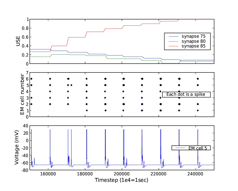
Figure 1. Creating publication-ready charts is easy using the matplotlib package.
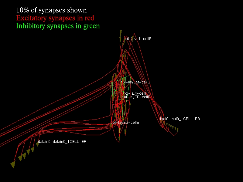
Figure 2. For interactive experimentation with 3-D views, Brainlab offers an OpenGL interface.
Quite often, some experimentation with a number of network parameters is required in order to find a balanced brain model. For example, if a synaptic strength is too high or too low, the model may not function realistically. We have seen how Brainlab could help a modeler do a search for a good model by repeatedly running the same model with a varying parameter. But an even more powerful technique than that simple search is to use another inspiration from biology, evolution, to do a genetic search on the values of whole set of parameters. I have used Brainlab to do this sort of multiparameter search with a genetic algorithm (GA) module of my own design and also with the standard GA module of the Scientific Python package, SciPy.
Brainlab has made my complex experiments practical, perhaps even possible. At this point I can't imagine doing them any other way. In fact, if NCS were to be reimplemented from scratch, I would suggest a significant design change: the elimination of the intermediate NCS input text file format. This file format is just complex enough to require a parser and the associated implementation complexity, documentation burden and slowdown in the loading of brain models. At the same time, it is not nearly expressive enough to be usable directly for any but the simplest brain models. Instead, a scripting environment such as Python/Brainlab could be integrated directly into NCS, and the scripts could create structures in memory that are accessed directly from the NCS simulation engine. The resulting system would be extremely powerful and efficient, and the overall documentation burden would be reduced. This general approach should be applicable to many different problems in other areas of model building research.
This summer, NCS is going to be installed on a new 4,000-processor IBM BlueGene cluster at our sister lab, the Laboratory of Neural Microcircuitry of the Brain Mind Institute at the EPFL in Switzerland, in collaboration with lab director Henry Markram. Early tests show that we can achieve a nearly linear speedup in NCS performance with increasing cluster size, due to efficient programming and the highly parallel nature of synaptic connections in the brain. We hope that other researchers around the world will find NCS and Brainlab useful in the effort to model and understand the human brain.
Resources for this article: /article/8203.
Rich Drewes (drewes@interstice.com) is a PhD candidate in Biomedical Engineering at the University of Nevada, Reno.
