Kernel Korner - Analysis of the HTB Queuing Discipline
The Hierarchical Token Buckets (HTB) queuing discipline, part of the Linux set of traffic control functions, is a mechanism that provides QoS capabilities and is useful for fine-tuning TCP traffic flow. This article offers a brief overview of queuing discipline components and describes the results of several preliminary performance tests. Several configuration scenarios were set up within a Linux environment, and an Ixia device was used to generate traffic. This testing demonstrated that throughput accuracy can be manipulated and that the bandwidth range is accurate within a 2Mbit/s range. The test results demonstrated the performance and accuracy of the HTB queuing algorithms and revealed methods for improving traffic management.
The traffic control mechanism comes into play after an IP packet is queued for transmit on an output interface but before the packet actually is transmitted by the driver. Figure 1 shows where traffic control decisions are made in relation to packet transmission on the physical Ethernet and transport-layer protocols, such as UDP and TCP.
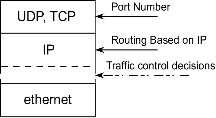
Figure 1. The kernel makes traffic control decisions after the packet is queued for transmit.
The traffic control kernel functionality, as implemented in Linux by Alexey Kuznetsov, includes four main components: queuing disciplines, classes of service, filters and policing.
Queuing disciplines are software mechanisms that define the algorithms used for treating queued IP packets. Each network device is associated with a queuing discipline, and a typical queuing discipline uses the FIFO algorithm to control the queued packets. The packets are stored in the order received and are queued as fast as the device associated with the queue can send them. Linux currently supports various queuing disciplines and provides ways to add new disciplines.
A detailed description of queuing algorithms can be found on the Internet at “Iproute2+tc Notes” (see the on-line Resources). The HTB discipline uses the TBF algorithm to control the packets queued for each defined class of service associated with it. The TBF algorithm provides traffic policing and traffic-shaping capabilities. A detailed description of the TBF algorithm can be found in the Cisco IOS Quality of Service Solutions Configuration Guide (see “Policing and Shaping Overview”).
A class of service defines policing rules, such as maximum bandwidth or maximum burst, and it uses the queuing discipline to enforce those rules. A queuing discipline and a class are tied together. Rules defined by a class must be associated with a predefined queue. In most cases, every class owns one queue discipline, but it also is possible for several classes to share the same queue. In most cases when queuing packets, the policing components of a specific class discard packets that exceed a certain rate (see “Policing and Shaping Overview”).
Filters define the rules used by the queuing discipline. The queuing discipline in turn uses those rules to decide to which class it needs to assign incoming packets. Every filter has an assigned priority. The filters are sorted in ascending order, based on their priorities. When a queue discipline has a packet for queuing, it tries to match the packet to one of the defined filters. The search for a match is done using each filter in the list, starting with the one assigned the highest priority. Each class or queuing discipline can have one or more filters associated with it.
Policing components make sure that traffic does not exceed the defined bandwidth. Policing decisions are made based on the filter and the class-defined rules. Figure 2 shows the relationship among all the components in the Linux traffic control mechanism.
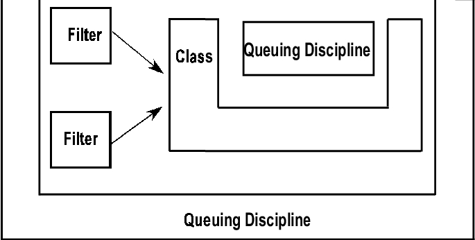
Figure 2. Linux traffic control mechanisms include queuing disciplines, classes, filters and policing.
TC is a user-level program that creates queues, classes and filters and associates them with an output interface (see “tc—Linux QoS control tool” in Resources). The filters can be set up based on the routing table, u32 classifiers and TOS classifiers. The program uses netlink sockets in order to communicate with the kernel's networking system functions. Table 1 lists the three main functions and their corresponding TC commands. See the HTB Linux Queuing Discipline User Guide for details regarding TC command options.
Table 1. TC Tool Functions and Commands
| TC Function | Command |
|---|---|
| tc qdisc | Create a queuing discipline. |
| tc filter | Create a filter. |
| tc class | Create a class. |
The HTB mechanism offers one way to control the use of the outbound bandwidth on a given link. To use the HTB facility, it should be defined as the class and the queuing discipline type. HTB shapes the traffic based on the TBF algorithm, which does not depend on the underlying bandwidth. Only the root queuing discipline should be defined as an HTB type; all the other class instances use the FIFO queue (default). The queuing process always starts at the root level and then, based on rules, decides which class should receive the data. The tree of classes is traversed until a matched leaf class is found (see “Hierarchical Token Bucket Theory”).
In order to test the accuracy and performance of the HTB, we used the following pieces of network equipment: one Ixia 400 traffic generator with a 10/100 Mbps Ethernet load module (LM100TX3) and one Pentium 4 PC (1GB RAM, 70GB hard drive) running a 2.6.5 Linux kernel. Two testing models were designed, one to test policing accuracy and one to test bandwidth sharing.
The first model (Figure 3) was used for testing the policing accuracy of a specific defined class. Port 1 in the Ixia machine generated traffic sent to IP 192.168.10.200 from one or more streams. The Linux machine routed the packets to interface eth0 (static route) and then sent them back to the Ixia machine on Port 2. All of the traffic control attributes were defined on the eth0 interface. All of the analysis was completed based on traffic results captured on Port 2 (the Ixia machine).
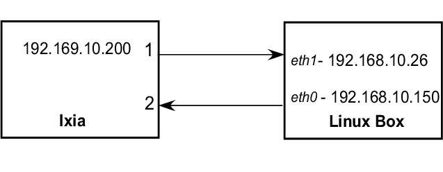
Figure 3. Test Model #1 Configuration
The second model (Figure 4) was used to test the way the bandwidth of two streams from the same class is shared. In this case, another two Ixia ports for transmitting data were used.
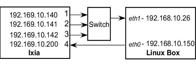
Figure 4. Test Model #2 Configuration
Port 1, Port 2 and Port 3 in the Ixia machine generated traffic sent to IP 192.168.10.200, each using one stream. The Linux machine routed those packets to interface eth0 based on a static route and then sent them back to the Ixia machine on Port 2. Traffic control attributes were defined on the eth0 interface. All analysis was done based on the traffic result captures on Port 2 (Ixia machine).
In all of the tests, the sending ports transmitted continuous bursts of packets on a specified bandwidth. The Ixia 10/100 Mbps Ethernet load module (model LM100TX3) has four separate ports, and each port can send up to 100Mbit/s. The Ixia load module provided support for generating multiple streams in one port but with one limitation: it couldn't mix the streams together and served only one stream at a time. This limitation exists because the scheduler works in a round-robin fashion. It sends a burst of bytes from stream X, moves to the next stream and then sends a burst of bytes from stream Y.
In order to generate a specific bandwidth from a stream, which is part of a group of streams defined in one port, specific attributes of the Ixia machine's configuration had to be fine-tuned. The attributes that required fine-tuning and their definitions are as follows:
Burst: the number of packets sent by each stream, before moving to serve the next stream.
Packet size: the size of a packet being sent by a stream.
Total bandwidth: the total bandwidth used by all streams.
See Table 2 for Ixia configuration details.
Table 2. Ixia Configuration
| Stream | Generated-Bandwidth | Packet Size | Burst Size |
|---|---|---|---|
| 1 | 15Mbit/s | 512B | 150 |
| 2 | 10Mbit/s | 512B | 100 |
| 3 | 2Mbit/s | 512B | 20 |
| Total | 27Mbit/s | – | – |
The goal was to determine the appropriate burst size that would achieve the requested generated bandwidth for each stream. Because all three streams used the same physical line, the way the data was sent on the line resembles the illustration in Figure 5.
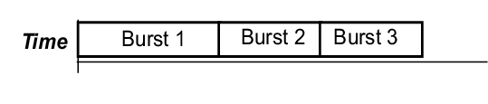
Figure 5. Data as sent on the line from the Ixia machine to the Linux system being tested.
The following equations define the relationship between the attributes:

Table 3 explains the variables used in the equation.
Table 3. Variables Used in the Attribute Relationship Equation
| Attribute | Definition |
|---|---|
| Tc | The sum of the times (in seconds) it takes to send bursts 1-i (Tc1 + Tc2 + Tc3+...). |
| Bs-i | The number of packets in a burst of stream i. |
| Ps-i | The size of packet sent by stream i. |
| Tb | The total bandwidth sent by all streams (bits/sec). |
| Nc | The number of Tc bursts in one second. |
| Bn-i | The requested bandwidth of stream i (bits/sec). |
Assuming that the packet size is the same for all streams, as in the example, the remaining calculation is that of the burst size.
Because all the streams share the same bandwidth, the requested burst values can be found by examining the ratios between the requested bandwidths, using the equation Bs-i = Bn-i. This number could be unusually large, though, so it can be divided until a reasonable value is obtained. In order to have different packet sizes defined for each stream, the burst size values can be altered until the required bandwidth is obtained for each stream. A spreadsheet program simplifies the calculation of multiple bandwidths.
When defining the HTB configuration, the following options of the tc class commands were used in order to achieve the required results:
rate = the maximum bandwidth a class can use without borrowing from other classes.
ceiling = the maximum bandwidth that a class can use, which limits how much bandwidth the class can borrow.
burst = the amount of data that could be sent at the ceiling speed before moving to serve the next class.
cburst = the amount of data that could be sent at the wire speed before moving to serve the next class.
Most of the traffic in the Internet world is generated by TCP, so packet sizes representative of datagram sizes, such as 64 (TCP Ack), 512 (FTP) and 1,500, were included for all test cases.

Figure 6. Test 1: One Stream In, One Stream Out
Table 4. Results for Testing Model 1
| Burst (Bytes) | Cburst (Bytes) | Packet-Size (Bytes) | In-Bandwidth (Mbit/s) | Out-Bandwidth (Mbit/s) |
|---|---|---|---|---|
| Default | Default | 128 | 40 | 33.5 |
| Default | Default | 64 | 40 | 22 (Linux halt) |
| Default | Default | 64 | 32 (Max) | 29.2 |
| 15k | 15k | 64 | 32 (Max) | 30 |
| 15k | 15k | 512 | 32 & 50 & 70 | 25.3 |
| 15k | 15k | 1,500 | 32 & 50 & 70 | 25.2 |
| 18k | 18k | 64 | 32 (Max) | 29.2 |
| 18k | 18k | 512 | 32 & 50 & 70 | 30.26 |
| 18k | 18k | 1,500 | 32 & 50 & 70 | 29.29 |
From the results in Table 4, the following statements can be made:
The maximum bandwidth a Linux machine can forward (receive on one interface and transmit on another interface) with continuous streams of 64-byte packets, is approximately 34Mbit/s.
The burst/cburst values, which give the most average accuracy results, are 18k/18k.
A linear relation exists between the burst value and the requested rate value. This relationship becomes apparent across tests.
The amount of bandwidth pushed on the output interface doesn't affect the accuracy of the results.
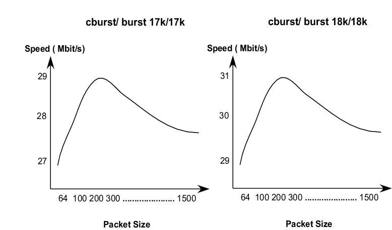
Figure 7. Graphic Analysis of Packet Size vs. Output Bandwidth
Figure 7 illustrates the relationship between packet size and output bandwidth after testing various packet sizes. From the results in Table 4 and Figure 7, we can conclude two things: throughput accuracy can be controlled by changing the cburst/burst values and the accuracy bandwidth range size is 2Mbit/s when using packets of sizes between 64 and 1,500 bytes. To verify that a linear relationship exists between the burst/cbursts values and the rate bandwidth, multiple burst and cburst values were tested. Table 5 shows the significant portion of the sampled data from the test case.
Table 5. Relationship between Burst/Cburst and Rate Values
| Burst (Bytes) | Cburst (Bytes) | Packet-Size (Bytes) | In-Bandwidth (Mbit/s) | Out-Bandwidth (Mbit/s) | Assigned-Rate (Mbit/s) |
|---|---|---|---|---|---|
| 9k | 9k | 64 | 32 | 17.5 | 15 |
| 9k | 9k | 512 | 32 | 15.12 | 15 |
| 9k | 9k | 1,500 | 32 | 15.28 | 15 |
| 4.8k | 4.8k | 64 | 32 | 8.96 | 8 |
| 4.8k | 4.8k | 512 | 32 | 8.176 | 8 |
| 4.8k | 4.8k | 1,500 | 32 | 8 | 8 |
| 3k | 3k | 64 | 32 | 17.5 | 15 |
| 3k | 3k | 512 | 32 | 15.12 | 15 |
| 3k | 3k | 1,500 | 32 | 15.28 | 15 |
18k/18k values were used as a starting point. The burst/cburst values were obtained by using the formula cburst/burst (Kbytes) = 18/(30M/Assign rate). From the results in Table 5, cburst/burst values can be defined dynamically for the rate value, such as when assuming a linear relationship.

Figure 8. Test 2: Three Streams In, One Stream Out
Table 6. Test 2 Results
| Stream | Burst (Bytes) | Cburst (Bytes) | Packet-Size (Bytes) | In-Bandwidth (Mbit/s) | Out-Bandwidth (Mbit/s) | Class |
|---|---|---|---|---|---|---|
| 1 | 17k | 17k | 64 | 15 | 12.7 | 3 |
| 2 | 17k | 17k | 512 | 20 | 17.1 | 3 |
| 3 | 1k | 1k | 512 | 4 | 2.01 | 2 |
| Total | 18k | 18k | – | 39 | 31.8 | – |
Table 6 shows an example of one level of inheritance. Class 2 and class 3 inherit the rate limit specification from class 1 (30Mbit/sec). In this test, the rate ceiling of the child classes is equal to the parent's rate limit, so class 2 and class 3 can borrow up to 30Mbit/sec. The linear relation assumption was used to calculate the cburst/burst values of all classes, based on their desired bandwidth.
Table 6 describes how the linear relationship works in the case of one level of inheritance. In this test, the input stream transmits continuous traffic of 39Mbit/s, and the accumulated output bandwidth is 31.8Mbit/s.
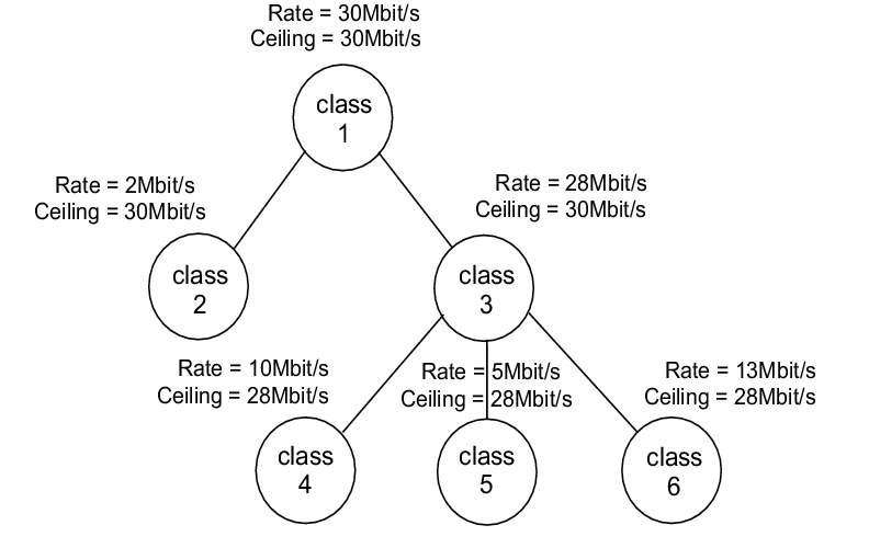
Figure 9. Test 3: Four Streams in, One Stream out
Table 7. Test 3 Results
| Stream | Burst (Bytes) | Cburst (Bytes) | Packet-Size (Bytes) | In-Bandwidth (Mbit/s) | Out-Bandwidth (Mbit/s) | Class |
|---|---|---|---|---|---|---|
| 1 | 1k | 1k | 512 | 5 | 2.04 | 2 |
| 2 | 6k | 6k | 6 | 15 | 11.326 | 4 |
| 3 | 3k | 3k | 64 | 10 | 5.67 | 5 |
| 4 | 7.8k | 7.8k | 512 | 20 | 13.02 | 6 |
| Total | 18k | 18k | – | 50 | 32.05 | – |
Table 7 shows the case of two levels of inheritance. Class 2 and class 3 inherit the rate limit specification from class 1 (30Mbit/s). Classes 4, 5 and 6 inherit the rate limit of class 3 (28Mbit/s) and share it based on their own rate limit specifications. In this test, the rate ceiling of the child classes is equal to the parent's rate limit, so classes 4, 5 and 6 can borrow up to 28Mbit/s. The linear relation assumption was used for calculating the cburst/burst values of all classes, based on their desired bandwidth.
From the results of Table 7, it can be observed that the linear relationship works in the case of two levels of inheritance. In this test the input port transmits continuous traffic of 50Mbit/s, and the accumulated output bandwidth is 32.05Mbit/s.

Figure 10. Test 1: Three streams In, one stream Out
Table 8. Test 1 Results
| Stream | Burst (Bytes) | Cburst (Bytes) | Packet-Size (Bytes) | In-Bandwidth (Mbit/s) | Out-Bandwidth (Mbit/s) | Class |
|---|---|---|---|---|---|---|
| 1 | 1k | 1k | 512 | 5 | 0.650 | 2 |
| 2 | 1k | 1k | 512 | 5 | 0.600 | 2 |
| 3 | 1k | 1k | 512 | 5 | 0.568 | 2 |
| Total | 18k | 18k | – | 15 | 1.818 | – |
As shown in Table 8, the bandwidth is distributed evenly when several streams are transmitting the same number of bytes and belong to the same class. Another test, in which the input bandwidth in stream 1 was higher than that of streams 2 and 3, showed that the output bandwidth of stream 1 also was higher than streams 2 and 3. From these results, it can be concluded that if more data is sent on a specific stream, the stream is able to forward more packets than other streams within the same class.
The test cases presented here demonstrate one way to evaluate HTB accuracy and performance. Although continuous packet bursts at a specific rate don't necessarily simulate real-world traffic, it does provide basic guidelines for defining the HTB classes and their associated attributes.
The following statements summarize the test case results:
The maximum bandwidth that a Linux machine can forward (receive on one interface and transmit on another interface) with continuous streams of 64-byte packets is approximately 34Mbit/s. This upper limit occurs because every packet that the Ethernet driver receives or transmits generates an interrupt. Interrupt handling occupies CPU time, and thus prevents other processes in the system from operating properly.
When setting the traffic rate to 30Mbit/s, the cburst/burst values, which give the most average accuracy results, are 18k/18k.
There is a linear relationship between the burst value and the requested rate. The cburst/burst values of a 30Mbit/s rate can be used as a starting point for calculating the burst values for other rates.
It is possible to control the throughput accuracy by changing the cburst/burst values. The accuracy bandwidth range size is approximately 2Mbit/s for 64–1,500 byte packet sizes.
Bandwidth is distributed evenly when several streams are transmitting the same number of bytes and belong to the same class.
Resources for this article: www.linuxjournal.com/article/7970.
Yaron Benita is originally from Jerusalem, Israel, and currently lives in San Francisco, California. He is the CMTS software manager at Prediwave. He works mostly in the networking and embedded fields. He is married and has a lovely six-month-old daughter. He can be reached at yaronb@prediwave.com or ybenita@yahoo.com.