
Optimization in GCC
In this article, we explore the optimization levels provided by the GCC compiler toolchain, including the specific optimizations provided in each. We also identify optimizations that require explicit specifications, including some with architecture dependencies. This discussion focuses on the 3.2.2 version of gcc (released February 2003), but it also applies to the current release, 3.3.2.
Let's first look at how GCC categorizes optimizations and how a developer can control which are used and, sometimes more important, which are not. A large variety of optimizations are provided by GCC. Most are categorized into one of three levels, but some are provided at multiple levels. Some optimizations reduce the size of the resulting machine code, while others try to create code that is faster, potentially increasing its size. For completeness, the default optimization level is zero, which provides no optimization at all. This can be explicitly specified with option -O or -O0.
The purpose of the first level of optimization is to produce an optimized image in a short amount of time. These optimizations typically don't require significant amounts of compile time to complete. Level 1 also has two sometimes conflicting goals. These goals are to reduce the size of the compiled code while increasing its performance. The set of optimizations provided in -O1 support these goals, in most cases. These are shown in Table 1 in the column labeled -O1. The first level of optimization is enabled as:
gcc -O1 -o test test.c
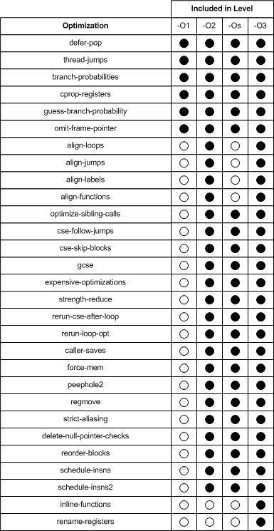
Table 1. GCC optimizations and the levels at which they are enabled.
Any optimization can be enabled outside of any level simply by specifying its name with the -f prefix, as:
gcc -fdefer-pop -o test test.c
We also could enable level 1 optimization and then disable any particular optimization using the -fno- prefix, like this:
gcc -O1 -fno-defer-pop -o test test.c
This command would enable the first level of optimization and then specifically disable the defer-pop optimization.
The second level of optimization performs all other supported optimizations within the given architecture that do not involve a space-speed trade-off, a balance between the two objectives. For example, loop unrolling and function inlining, which have the effect of increasing code size while also potentially making the code faster, are not performed. The second level is enabled as:
gcc -O2 -o test test.c
Table 1 shows the level -O2 optimizations. The level -O2 optimizations include all of the -O1 optimizations, plus a large number of others.
The special optimization level (-Os or size) enables all -O2 optimizations that do not increase code size; it puts the emphasis on size over speed. This includes all second-level optimizations, except for the alignment optimizations. The alignment optimizations skip space to align functions, loops, jumps and labels to an address that is a multiple of a power of two, in an architecture-dependent manner. Skipping to these boundaries can increase performance as well as the size of the resulting code and data spaces; therefore, these particular optimizations are disabled. The size optimization level is enabled as:
gcc -Os -o test test.c
In gcc 3.2.2, reorder-blocks is enabled at -Os, but in gcc 3.3.2 reorder-blocks is disabled.
The third and highest level enables even more optimizations (Table 1) by putting emphasis on speed over size. This includes optimizations enabled at -O2 and rename-register. The optimization inline-functions also is enabled here, which can increase performance but also can drastically increase the size of the object, depending upon the functions that are inlined. The third level is enabled as:
gcc -O3 -o test test.c
Although -O3 can produce fast code, the increase in the size of the image can have adverse effects on its speed. For example, if the size of the image exceeds the size of the available instruction cache, severe performance penalties can be observed. Therefore, it may be better simply to compile at -O2 to increase the chances that the image fits in the instruction cache.
The optimizations discussed thus far can yield significant improvements in software performance and object size, but specifying the target architecture also can yield meaningful benefits. The -march option of gcc allows the CPU type to be specified (Table 2).
Table 2. x86 Architectures
| Target CPU Types | -march= Type |
|---|---|
| i386 DX/SX/CX/EX/SL | i386 |
| i486 DX/SX/DX2/SL/SX2/DX4 | i486 |
| 487 | i486 |
| Pentium | pentium |
| Pentium MMX | pentium-mmx |
| Pentium Pro | pentiumpro |
| Pentium II | pentium2 |
| Celeron | pentium2 |
| Pentium III | pentium3 |
| Pentium 4 | pentium4 |
| Via C3 | c3 |
| Winchip 2 | winchip2 |
| Winchip C6-2 | winchip-c6 |
| AMD K5 | i586 |
| AMD K6 | k6 |
| AMD K6 II | k6-2 |
| AMD K6 III | k6-3 |
| AMD Athlon | athlon |
| AMD Athlon 4 | athlon |
| AMD Athlon XP/MP | athlon |
| AMD Duron | athlon |
| AMD Tbird | athlon-tbird |
The default architecture is i386. GCC runs on all other i386/x86 architectures, but it can result in degraded performance on more recent processors. If you're concerned about portability of an image, you should compile it with the default. If you're more interested in performance, pick the architecture that matches your own.
Let's now look at an example of how performance can be improved by focusing on the actual target. Let's build a simple test application that performs a bubble sort over 10,000 elements. The elements in the array have been reversed to force the worst-case scenario. The build and timing process is shown in Listing 1.
Listing 1. Effects of Architecture Specification on a Simple Application
[mtj@camus]$ gcc -o sort sort.c -O2
[mtj@camus]$ time ./sort

real    0m1.036s
user    0m1.030s
sys     0m0.000s
[mtj@camus]$ gcc -o sort sort.c -O2 -march=pentium2
[mtj@camus]$ time ./sort

real    0m0.799s
user    0m0.790s
sys     0m0.010s
[mtj@camus]$
By specifying the architecture, in this case a 633MHz Celeron, the compiler can generate instructions for the particular target as well as enable other optimizations available only to that target. As shown in Listing 1, by specifying the architecture we see a time benefit of 237ms (23% improvement).
Although Listing 1 shows an improvement in speed, the drawback is that the image is slightly larger. Using the size command (Listing 2), we can identify the sizes of the various sections of the image.
Listing 2. Size Change of the Application from Listing 1
[mtj@camus]$ gcc -o sort sort.c -O2
[mtj@camus]$ size sort
   text    data     bss     dec     hex filename
    842     252       4    1098     44a sort
[mtj@camus]$ gcc -o sort sort.c -O2 -march=pentium2
[mtj@camus]$ size sort
   text    data     bss     dec     hex filename
    870     252       4    1126     466 sort
[mtj@camus]$
From Listing 2, we can see that the instruction size (text section) of the image increased by 28 bytes. But in this example, it's a small price to pay for the speed benefit.
Some specialized optimizations require explicit definition by the developer. These optimizations are specific to the i386 and x86 architectures. A math unit, for one, can be specified, although in many cases it is automatically defined based on the specification of a target architecture. Possible units for the -mfpmath= option are shown in Table 3.
Table 3. Math Unit Optimizations
| Option | Description |
|---|---|
| 387 | Standard 387 Floating Point Coprocessor |
| sse | Streaming SIMD Extensions (Pentium III, Athlon 4/XP/MP) |
| sse2 | Streaming SIMD Extensions II (Pentium 4) |
The default choice is -mfpmath=387. An experimental option is to specify both sse and 387 (-mfpmath=sse,387), which attempts to use both units.
In the second optimization level, we saw that a number of alignment optimizations were introduced that had the effect of increasing performance but also increasing the size of the resulting image. Three additional alignment optimizations specific to this architecture are available. The -malign-int option allows types to be aligned on 32-bit boundaries. If you're running on a 16-bit aligned target, -mno-align-int can be used. The -malign-double controls whether doubles, long doubles and long-longs are aligned on two-word boundaries (disabled with -mno-align-double). Aligning doubles provides better performance on Pentium architectures at the expense of additional memory.
Stacks also can be aligned by using the option -mpreferred-stack-boundary. The developer specifies a power of two for alignment. For example, if the developer specified -mpreferred-stack-boundary=4, the stack would be aligned on a 16-byte boundary (the default). On the Pentium and Pentium Pro targets, stack doubles should be aligned on 8-byte boundaries, but the Pentium III performs better with 16-byte alignment.
For applications that utilize standard functions, such as memset, memcpy or strlen, the -minline-all-stringops option can increase performance by inlining string operations. This has the side effect of increasing the size of the image.
Loop unrolling occurs in the process of minimizing the number of loops by doing more work per iteration. This process increases the size of the image, but it also can increase its performance. This option can be enabled using the -funroll-loops option. For cases in which it's difficult to understand the number of loop iterations, a prerequisite for -funroll-loops, all loops can be unrolled using the -funroll-all-loops optimization.
A useful option that has the disadvantage of making an image difficult to debug is -momit-leaf-frame-pointer. This option keeps the frame pointer out of a register, which means less setup and restore of this value. In addition, it makes the register available for the code to use. The optimization -fomit-frame-pointer also can be useful.
When operating at level -O3 or having -finline-functions specified, the size limit of the functions that may be inlined can be specified through a special parameter interface. The following command illustrates capping the size of the functions to inline at 40 instructions:
gcc -o sort sort.c --param max-inline-insns=40
This can be useful to control the size by which an image is increased using -finline-functions.
The default stack alignment is 4, or 16 words. For space-constrained systems, the default can be minimized to 8 bytes by using the option -mpreferred-stack-boundary=2. When constants are defined, such as strings or floating-point values, these independent values commonly occupy unique locations in memory. Rather than allow each to be unique, identical constants can be merged together to reduce the space that's required to hold them. This particular optimization can be enabled with -fmerge-constants.
Depending on the specified target architecture, certain other extensions are enabled. These also can be enabled or disabled explicitly. Options such as -mmmx and -m3dnow are enabled automatically for architectures that support them.
We've discussed many optimizations and compiler options that can increase performance or decrease size. Let's now look at some fringe optimizations that may provide a benefit to your application.
The -ffast-math optimization provides transformations likely to result in correct code but it may not adhere strictly to the IEEE standard. Use it, but test carefully.
When global common sub-expression elimination is enabled (-fgcse, level -O2 and above), two other options may be used to minimize load and store motions. Optimizations -fgcse-lm and -fgcse-sm can migrate loads and stores outside of loops to reduce the number of instructions executed within the loop, therefore increasing the performance of the loop. Both -fgcse-lm (load-motion) and -fgcse-sm (store-motion) should be specified together.
The -fforce-addr optimization forces the compiler to move addresses into registers before performing any arithmetic on them. This is similar to the -fforce-mem option, which is enabled automatically in optimization levels -O2, -Os and -O3.
A final fringe optimization is -fsched-spec-load, which works with the -fschedule-insns optimization, enabled at -O2 and above. This optimization permits the speculative motion of some load instructions to minimize execution stalls due to data dependencies.
Earlier we used the time command to identify how much time was spent in a given command. This can be useful, but when we're profiling our application, we need more insight into the image. The gprof utility provided by GNU and the GCC compiler meets this need. Full coverage of gprof is outside the scope of this article, but Listing 3 illustrates its use.
Listing 3. Simple Example of gprof
[mtj@camus]$ gcc -o sort sort.c -pg -O2 -march=pentium2
[mtj@camus]$ ./sort
[mtj@camus]$ gprof --no-graph -b ./sort gmon.out
Flat profile:

Each sample counts as 0.01 seconds.
  %   cumulative   self              self     total
 time   seconds   seconds    calls  ms/call  ms/call  name
100.00      0.79     0.79        1   790.00   790.00  bubbleSort
  0.00      0.79     0.00        1     0.00     0.00  init_list
[mtj@camus]$
The image is compiled with the -pg option to include profiling instructions in the image. Upon execution of the image, a gmon.out file results that can be used with the gprof utility to produce human-readable profiling data. In this use of gprof, we specify the -b and --no-graph options. For brief output (excludes the verbose field explanations), we specify -b. The --no-graph option disables the emission of the function call-graph; it identifies which functions call which others and the time spent on each.
Reading the example from Listing 3, we can see that bubbleSort was called once and took 790ms. The init_list function also was called, but it took less than 10ms to complete (the resolution of the profile sampling), so its value was zero.
If we're more interested in changes in the size of the object than speed, we can use the size command. For more specific information, we can use the objdump utility. To see a list of the functions in our object, we can search for the .text sections, as in:
objdump -x sort | grep .text
From this short list, we can identify the particular function we're interested in understanding better.
The GCC optimizer is essentially a black box. Options and optimization flags are specified, and the resulting code may or may not improve. When they do improve, what exactly happened within the resulting code? This question can be answered by looking at the resulting code.
To emit target instructions from the compiler, the -S option can be specified, such as:
gcc -c -S test.c
which tells gcc to compile the source only (-c) but also to emit assembly code for the source (-S). The resulting assembly output will be contained in the file test.s.
The disadvantage of the previous approach is you see only assembly code, no aspect of the size of the actual instructions is given. For this, we can use objdump to emit both assembly and native instructions, like so:
gcc -c -g test.c
objdump -d test.o
For gcc, we specify compile with only -c, but we also want to include debug information in the object (-g). Using objdump, we specify the -d option to disassemble the instructions in the object. Finally, we can get assembly-interspersed source listings with:
gcc -c -g -Wa,-ahl,-L test.c
This command uses the GNU assembler to emit the listing. The -Wa option is used to pass the -ahl and -L options to the assembler to emit a listing to standard-out that contains the high-level source and assembly. The -L option retains the local symbols in the symbol table.
All applications are different, so there's no magic configuration of optimization and option switches that yield the best result. The simplest way to achieve good performance is to rely on the -O2 optimization level; if you're not interested in portability, specify the target architecture using -march=. For space-constrained applications, the -Os optimization level should be considered first. If you're interested in squeezing the most performance out of your application, your best bet is to try out the different levels and then use the various utilities to check the resulting code. Enabling and/or disabling certain optimizations also may help exploit the optimizer to receive the best performance.
Resources for this article: www.linuxjournal.com/article/7971.
M. Tim Jones (mtj@mtjones.com) is a senior principal engineer with Emulex Corp. in Longmont, Colorado. In addition to being an embedded firmware engineer, Tim recently finished writing the book BSD Sockets Programming from a Multilanguage Perspective. He has written kernels for communications and research satellites and now develops embedded firmware for networking products.
