The Linux Trace Toolkit
As recent Linux history has shown (Mindcraft, anyone?), performance is not only good publicity, it's important. Yet current means of measuring performance offer only global statistics about the whole system or very precise data about an isolated application. Moreover, these often fail in helping the programmer or the system administrator to isolate a performance bottleneck resulting from the interaction of complex internetworking applications, which are more and more common. The Linux Trace Toolkit (LTT) addresses these issues and provides users with a unique view of the system's behavior with minimal performance overhead (< 2.5%).
In order to be extendable and accomplish its task without hindering system performance, LTT is designed to be as modular as possible. In fact, it would be wrong to call it a “tool” since it is composed of many pieces that, grouped together, fulfill the desired function. This toolkit is implemented in four parts. First, there is a Linux kernel that enables events to be logged. Second, a Linux kernel module takes care of storing the events into its buffer and then signals the trace daemon when it reaches a certain threshold. The latter then reads the data from the module, which is visible from user space as a character device. Last, but certainly not least, the data decoder takes the raw trace data and puts it in a human-readable format while performing some basic and more advanced analysis. This decoder, as will be discussed further, serves as the toolkit's graphic and command-line front end.
The LTT tar.gz archive can be found at http://www.opersys.com/LTT/ and contains the following items:
Copying: the GNU GPL License
Help: LTT's help files in an HTML-browsable format
TraceDaemon: the directory containing the trace daemon
TraceToolkit: the directory containing the trace toolkit front end
patch-ltt-kernelversion-yymmdd: the kernel patch of yymmdd kernelversion
trace: a script to start the trace daemon
tracecpuid: another script to start the trace daemon
tracedump: a script to dump the content of trace
traceanalyze: a script to analyze a trace
traceview: a script to view a trace in graphical form
The scripts are there to speed up the tools' most common usages, but the tools can be summoned directly without any script.
To install LTT, simply follow the instructions that come with the LTT package. The first and hardest step is patching the kernel. Once this is done, configure the kernel and compile it. Note that there is an option for compiling with or without the tracing code. When compiled without, the resulting kernel operates as if you hadn't applied any patch to it. Next, compile the trace daemon and the trace toolkit graphic front end and put them in your favorite directory (/usr/bin or /usr/local/bin for example). Reboot with the LTT patched kernel, and you're ready to go.
To demonstrate the toolkit's operation, we traced 10 seconds' worth of system operation. During those 10 seconds, two commands were issued: dir on a directory not accessed since system boot (i.e., not present in the dcache) and bzip2 on a 10MB file. The system was booted in single-user mode (in order to have as few applications running as possible, and therefore isolate the operation of the observed applications) using the modified kernel. Note that no events are recorded by the kernel module until the trace daemon has issued the start command to it using the ioctl system call. The following command was issued to start the tracing:
trace 10 out140
trace is a script that takes two arguments: the number of seconds the trace should last and the base name for the output file. Two files are produced: out140.trace and out140.proc. The former holds the data recorded by the kernel module, and the latter, the content of /proc when the trace started. Using these two files, we know what the system looked like before we started tracing it and what happened during the trace. Hence, we can reconstruct the system's behavior.
Note that the trace daemon accepts many command-line options used to configure the kernel trace module. For instance, one can specify the events to be traced and the desired level of details. One can also specify whether CPU IDs should be recorded for SMP machines. Since LTT fetches the calling address for system calls, you can specify at which calling depth this address should be fetched or which address range it is a part of.
This is the most interesting part about LTT and what differentiates it from other tools. Even though the current example is rather simplistic, more elaborate traces can be generated and analyzed just as easily. To view the trace in the graphical front end, simply type:
traceview out140
The traceview script accepts one argument: the base name of the generated trace. It then executes the trace toolkit front end, passing it the out140.trace and out140.proc files. Note that the front end can be invoked manually and can be used as a command-line tool as well. In the latter case, it can be used to dump the contents of trace in a human-readable format or perform a detailed trace analysis. The complete options are described in the documentation included with LTT.
A sample display of the front end can be seen in Figure 1. As usual, there is a menu, a toolbar and the data. To present the data, the tool uses three thumbnails. The first, Event Graph, presents the events in a graphical way. On the left, a list of all processes that existed during the trace is presented. On the right, a scrollable graph displays the transitions that marked the time frame being displayed. A vertical transition means the flow of control has been passed to another entity. The color of the vertical line used for the transitions indicates the type of event that caused the transition. Blue is for a system call, grey for a trap and white for an interrupt. Horizontal lines indicate the time spent executing code belongs to the entity in the process list at the same height. A green line is for application code and an orange line is for kernel code.
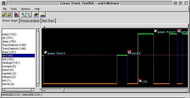
Figure 1. LTT Front End
In Figure 1, we can see that sh was running and a page fault occurred. Control was transfered to the kernel, which did some operations and then gave control back to sh. The latter executed for a while, then did a wait4 system call. This, in turn, gave control back to the kernel. After a couple of operations, the kernel decided to do a task switch and handed control to process 152, bzip2. While bzip2 was running, another trap occurred. Toward the end of the trace, we can see bzip2 made a system call to getpid, and on returning, continued executing.
Figure 2 presents a more interesting case. For illustration purposes, the trace portion was zoomed out; some icons overlap, but the meaning is fairly straightforward. Here, bzip2 tries to read something, but the kernel doesn't find it. bzip2 starts waiting for I/O (input/output) and the kernel schedules the idle task. Two milliseconds later, the hard disk sends an interrupt to signal that it finished reading (that's the icon with a chip and an exclamation mark with a 14 beside it, 14 being the IDE disk IRQ). bzip2 is then rescheduled, stops waiting for I/O and returns to its normal execution. Here, we can see exactly how much time bzip2 spent waiting for I/O and the exact chronology of events that led to it losing CPU control and regaining it. When trying to comprehend complex interactions between tasks, this type of information can make all the difference.
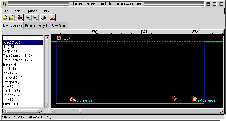
Figure 2. Event Graph
Giving a different perspective, the second thumbnail, Process Analysis, provides us with an in-depth analysis of each process that existed during the trace and a global analysis of the system. Figure 3 presents a sample of this analysis. On the left, the process tree is presented. At the top of the tree lies the idle task (PID 0) which is presented as being The All Mighty. Since the idle task never does anything worth tracing, it is used to present data about the whole system: trace start time, trace end time, duration, time spent idle (idle was scheduled as running). Then the number of occurrences of key events is presented. Notice some events given here can't be accounted for by using the information in /proc.
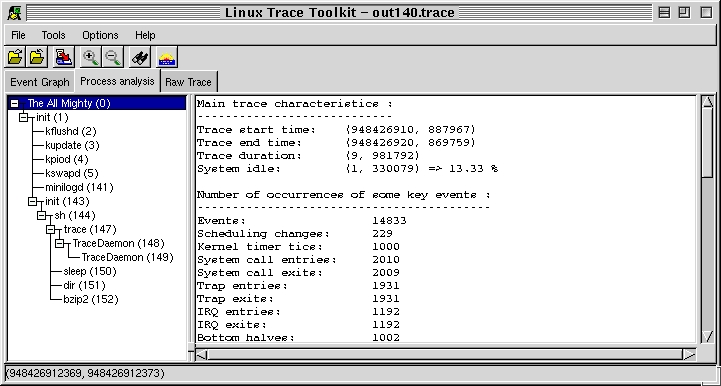
Figure 3. Process Analysis
When selecting dir and bzip2 processes, the information in Listing 1 is displayed. Notice the difference in percentages between the time running (time scheduled by the kernel as having control over the CPU) and the time spent actually executing code belonging to the application. In bzip2's case, the gap is very small, which accurately describes bzip2's behavior as CPU-intensive; whereas in dir's case, less than half of the time it was scheduled was spent executing its own code, the rest being spent in kernel routines.
Note also the differences between the time spent waiting for I/O and the time running. dir spent more time waiting for I/O than it spent executing. bzip2, on the other hand, spent little time waiting for I/O compared to the time it spent in running state. This information wasn't collected using sampling on the system clock, as is done currently for the information available through /proc. This information is calculated using the trace information and is therefore the exact information regarding the observed task.
Last but not least, the third thumbnail presents the raw trace. Figure 4 presents a portion of a raw trace. The events are presented in chronological order of occurrence. For each event, the following information is given: the CPU-ID of the processor on which it occurred, the event type, the exact time of occurrence (down to the microsecond), the PID of the task to which it belongs, the size of the entry in the kernel module that was taken in order to record the event in full and the description of the event. Notice how the address from which a system call was made is displayed. This could eventually be used to correlate with data recorded from within the application or simply to know which part of the code made the call. Unlike other tracing methods such as ptrace, there is no effect on the application's behavior, except the minimal event-data collection delays.
Figure 4. Portion of Raw Trace
As this article has shown, LTT is an effective tool for recording critical system information. Moreover, it is rather simple to use and the information presented is accessible to a large portion of the community. In an academic environment, LTT can be used in a course on operating systems, helping students get first hand experience with a live operating system and how it interacts with different applications.
Given its capabilities, modularity, extensibility and minimal overhead, we hope to see the tracing code become part of the mainstream Linux kernel soon (maybe not in 2.3/2.4 currently in feature freeze, but in the next development branch). Another possible application for LTT, which gathered a lot of interest, is to use it as part of a security auditing system with Tripwire-type capabilities. At the time of this writing, the authors know of at least one Linux distribution which plans to include LTT as part of their standard distribution.
Karim Yaghmour (karym@opersys.com) is an operating system freak. He's been playing around with OS internals for quite a while and has even written his own OS. He's currently completing his master's degree at the Ecole Polytechnique de Montréal, where the Linux Trace Toolkit is part of his research. He started his own consulting company, Opersys, Inc., that specializes in operating systems (http://www.opersys.com/) and offers expertise and courses on Linux internals and real-time derivatives.
Michel Dagenais (michel.dagenais@polymtl.ca) is a professor at Ecole Polytechnique de Montréal. He has authored or co-authored a large number of scientific publications in the fields of software engineering, structured documents on the Web and object-oriented distributed programming for collaborative applications.