
Portable Real-Time Applications
In today's visual world of data processing, many people think solving problems with computers means implementing graphical user interfaces (GUIs). From this point of view, writing real-time applications means writing GUIs while at the same time mastering the system-dependent functions that ensure predictable response times, often in conjunction with arcane hardware features. This mixture of system-dependent GUIs and hardware-dependent real-time functions usually leads to complex, expensive and non-portable applications. To attack the general problem of writing portable real-time applications, I will first look back at the roots of the UNIX operating system. Then, I will apply the lessons learned to a simple multimedia application that runs on three very different platforms: Linux, IRIX and Win32 (MS Windows 95/98/NT/2000).
Most people know how a sine or a square wave sounds. They can be heard as a beep or a test signal from a PC speaker, a telephone or a common musical instrument such as a flute. The portable application we will implement produces such sounds. Sine, triangle and square waves are just special cases of a more general wave produced by the Duffing oscillator (see Resources). Depending on the parameters, which can be adjusted by two sliders in the GUI, this oscillator is also able to emit chaotic sounds. (Chaotic, in this sense, gets its meaning from nonlinear dynamics or chaos theory.) When starting the application, you will actually be able to put some research results to the test by listening to the sound and by watching the graphical behaviour of the Duffing oscillator. Nonetheless, such an application has to produce sound continuously, otherwise the sound will be distorted by clicks or even silence. Thus, this application is an example of a real-time application.
Before starting our implementation, we must think about the design of such a portable application, forgetting for the moment that we want to implement our multimedia application with a GUI. Most UNIX programmers know what is meant by the UNIX philosophy. In the good old days, when all user interfaces were textual, not graphical, Kernighan and Pike explained this notion in the epilogue of their book The Unix Programming Environment. They emphasized the importance of breaking a problem into separate sub-problems with a simple interface between them, usually a pipe. Putting a pipe between the processes means having the textual output of one process read as textual input by the next process. Each sub-problem was then implemented and tested stepwise on its own, preferably by applying existing tools.
This design philosophy allows for writing portable applications and is a sharp contrast to today's development environments. Today, many programmers use some visual development environment to build monolithic applications bound to one platform.
The crucial question is: can a GUI-based real-time application be implemented as an old-fashioned UNIX pipeline? It can—you just have to choose the right tools. A GUI-based application which allows for adjustment of parameters, emission of sound and visualization of results can be broken down into a pipeline of processes: GUI-->Sound Generation-->Sound Output-->Graph.
Stage 1 (GUI) provides a way to interactively adjust the parameters of a mathematical model. These parameters may be adjusted with knobs, slide bars or with a point in a two-dimensional plane, whichever is most intuitive. It can easily be replaced without affecting other stages, provided it produces the same kind of data on its standard output.
Stage 2 (generation) is invisible to the user, so it does not need a GUI. It takes the parameters from stage 1 and processes them using a mathematical model of a physical process. The only challenge at this stage is doing both parameter input and continuous computation at the same time, but at different unsynchronized rates.
Stage 3 (sound emission) reads the resulting waveform and hands it over to the sound system. Because of significant differences in the implementation of sound systems on platforms like Linux, IRIX and Win32, we need to have some experience with encapsulating platform-dependent code. Fortunately, this is the only stage written for a particular platform.
Stage 4 (graphical output), just like stage 1, has contact with the user and will therefore be implemented as a GUI. Just like stage 1, the results can be represented in many different ways without affecting other stages. Examples are tables, simple amplitude diagrams, trajectories in phase space or Poincaré sections.
Each stage can also be used on its own or as a building block in a completely different application. Stage 3 is the most interesting building block.
It is clear that transferring large amounts of data from stage 2 to stage 3 is the bottleneck of the system. Writing into the pipe, reading again and scanning each sample absorbs more CPU time than every other operation. So, stages 2 and 3 must be integrated into one program, because passing of data (44,100 values per second) takes too much time. You might think integrating these stages into one is a design flaw—it is not. I could have easily renumbered stages and changed this article, but I preferred to show you how cruel life in real time is to ingenuous software designers.
For Stage 1, Tcl/Tk is a natural choice as a tool for implementation of the first sub-problem. Many people have forgotten that the GUI process in Tcl/Tk also has a textual standard output which can be piped into the second process.
In Stages 2 and 3, the sound generator reads the textual parameters from the GUI-process and computes the proper sound signal from it in real time. Therefore, it should be written in C, because it is the most critical sub-problem as far as real-time constraints are concerned. As a side effect of sound generation, the data needed for graphing the results will be written to standard output and piped into the final stage of the application.
Since Stage 4 outputs graphs of the results, it is also a task well-suited for a tool like Tcl/Tk.
The user will notice only stages 1 and 4 of the pipeline, because he can see each of them as a window and interact with them. It is an interesting paradox that the seemingly important stages 1 and 4 are rather trivial to implement, given a tool like Tcl/Tk. Stages 2 and 3, although mostly unnoticed, are the most challenging sub-problems because of synchronization concepts in real time (select or thread), real-time constraints due to continuous sound emission and the different handling of sound systems and all platform dependencies.
We have already mentioned that one advantage of this pipeline approach is splitting the development into largely independent sub-tasks, which allows one programmer to work on each task concurrently. Equally important is the fact that each stage could also be implemented in different ways by different programmers. To demonstrate this, we will look at three solutions to the stage 1 task:
Textual user interface on the command line
GUI with Tcl/Tk (Listings 1 and 2)
GUI with a Netscape browser and GNU AWK 3.1 as a server (Listing 3, which is not printed but is included in the archive file)
Also, we will look at three different implementations of stage 4:
Textual output into a file
Graphical output of this data with GNUPLOT (Figure 5)
Graphical output with Tcl/Tk (Listing 5)
Now that the design of the system is clear, it is time to become more precise about the type of sound we want to produce. Imagine a driven steel beam held pinned to fixed supports at the bottom and top. When driving the beam from the side, the fixed supports induce a membrane tension at finite deflections. This leads to a hardening nonlinear stiffness for moderately large deflections by a cubic term. At the beginning of this century, the engineer Georg Duffing from Berlin, Germany was annoyed by this kind of noise which came from vibrating machine parts. Such noise is not only a nuisance, it also shortens the expected lifetime of machine parts. Duffing found a simple nonlinear differential equation which describes the behaviour of machine parts under certain circumstances:
x'' + kx' + x3 = Bcos(t)
This oscillator is driven by a sinusoidal force on the right of the equation (with magnitude B) and damped by the parameter k on the left side of the equation. So, there are only two free parameters in this driven oscillator.

Figure 1. Changing parameters k (damping) and B (forcing) will move the oscillator in or out of a chaotic regime (see page 11, Thompson/Stewart).
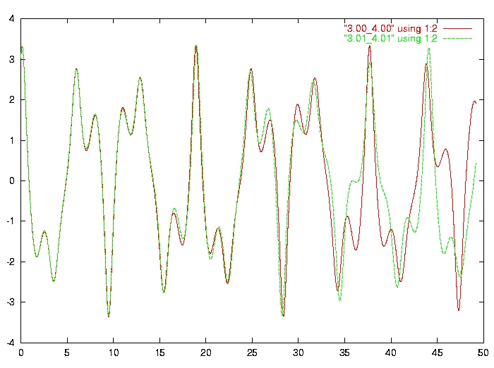
In Figure 3, you can see a short wave form originating from such a sound machine. Unlike Duffing, you can simulate the noise production with your computer by varying the parameters with a GUI such as the one shown in Figures 1 and 2. You should expect that varying parameter B on the right axis of figure 1 influences just the volume of the noise. In fact, by pushing B to its minimal position 0, you can actually switch off the noise. When pushing parameter B to its maximum, noise will not only become louder, it will also change the main frequency but not in a continuous and monotonic way. This strange behaviour of changing frequency along with loudness does not occur in linear oscillators. In 1980, Ueda published a systematic look at the points in the plane opened up by the parameters B and k in Figure 1. By computer simulation, he found areas where the oscillator emits chaotic sounds. These results are summarized in Thompson and Stewart's book (see Resources).
Why is it so hard to compute these wave forms? After all, a formula to be evaluated for each time instant should be all that is needed; however, there is no such analytical function. When in trouble, engineers often fall back on simple approximations. We will do so with a technique called Finite Differencing (see Resources) which gives us a one-line calculation at each time instant (Listing 4).
With Tcl/Tk, it is so simple to implement stage 1 that we can afford to look at two different implementations. When executing the script in Listing 2 with the wish -f duffing.tcl command, the two independent parameters k and B are visualized as the axes of a two-dimensional coordinate system. Drag the circle to any place on the map, and the new coordinates will be printed to standard output. But maybe you prefer the simpler implementation shown in Listing 1, which displays both parameters as scales. If you run a computer without a GUI, you can still work with the software presented here. In this case, forget about stage 1; stage 2 will read its input from the command line. Enter lines like k 0.05 or B 7.5 at run time, and stage 2 will not notice the difference.
Stages 2 and 3 had to be integrated into one program for reasons of efficiency. It was tempting to implement each stage as a single thread of execution. Threads of execution behave mostly like processes that share a single data space: one waiting for input to modify parameters, the other one calculating the wave form to be emitted. How does one implement threads of execution in a portable way? The POSIX thread library (see Resources) is now available for most operating systems, including the ones mentioned earlier. For example, at STN Atlas Elektronik we use threads for sound generation with multiple sound cards in a multiprocessor setting (two CPUs and Linux 2.2 SMP). As explained in David Butenhof's excellent book, threads make it very hard to debug software; therefore, we will refrain from using them here.

Figure 2. This user interface allows for precise tuning of parameters. Notice that you can actually hear chaotic regimes; they sound markedly “dirty” and not as “clean” as other regions.
Listing 4. Stage 2 and 3 in C, integrator.c
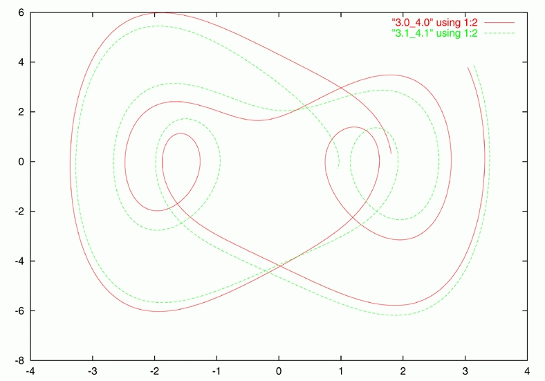
Fortunately, the problem of dealing with unsynchronized events can be solved with the often underestimated select system call (Listing 4, function main). The main loop of Listing 4 has a short loop to check whether there is data coming in from standard input. Then, it calculates a block of data by Finite Differencing and finally emits it. While calculating, some data points are printed to standard output. Only those which occur at integral multiples of the cycle period of the driving force, having the same phase angle, are printed. This technique of selecting data points to display is at the heart of the Poincaré section, a kind of stroboscope which reveals hidden order within chaotic data (Figure 5). Notice that this data is the input to stage 4.
Figure 3. The default parameters show sensitive dependence on initial conditions (see page 4, Thompson/Stewart).
This was the easy part; the hard part is handing over the data to the sound system in a portable way. In this respect, Linux is the platform handled most easily. Writing data to the special file /dev/dsp is enough. With IRIX, we also need just one function call; not the usual write, but a special sound function. In both cases, synchronization is implemented by the blocking behaviour of these functions. This is in contrast to Win32, which bothers the programmer with buffer handling, and synchronization must be done with callback functions. Using the new DirectSound API was not an option because Microsoft has failed to implement the DirectX API in Windows NT.
How to Compile and Run Listing 4
Listing 5. Stage 4 in Tcl/Tk, out.tcl
Stage 4 is, again, rather simple to implement (Listing 5, Figure 5). Each data point read is printed as a dot in the phase space diagram. When producing Poincaré section data as in stage 3, linear oscillators produce circles or spirals, degenerating into fixed points, which is rather boring. A chaotic oscillator is needed to plot the strange attractor shown in Figure 5.
Figure 4. High resolution Poincaré section of one chaotic attractor
In the sidebar “How to Compile and Run Listing 4”, you can see how to compile the stage 3 program on different platforms and how to start the whole application as a UNIX pipe. You might be surprised to find that the compiler gcc can be used even with the Win32 operating systems. How is this possible? The gcc for Win32 is part of a UNIX-compatible environment called the Cygwin Toolset (see Resources). It allows you to work with gcc and its friends on any Win32 operating system just as if it were a well-behaved UNIX system. Many GNU packages run out of the box with it. If you want to use the multimedia functions of Win32 (along with DirectX access) or the POSIX thread library, you must get and install them separately (see Resources). Since I started working on Win32, it became more and more important to adhere to the POSIX system calls, written down in the XPG4 set of standards. Doing so has become a rewarding habit, because it is the cornerstone of portability in the UNIX world.
What pleased me most was the possibility of installing gcc from the Cygwin Toolset as a cross compiler on my Linux 2.2 system. Now I can write and debug my software with Linux, no matter where it is supposed to run later. In the end, I compile it with the cross compiler and get a debugged Win32 executable. What an achievement! If you also would enjoy working this way, follow Mumit Khan's recipe for cooking a cross compiler (see Resources).
Jürgen Kahrs (Juergen.Kahrs@t-online.de) is a development engineer at STN Atlas Elektronik in Bremen, Germany. There, he uses Linux for generating sound in educational simulators. He likes old-fashioned tools such as GNU AWK and Tcl/Tk. He also did the initial work for integrating TCP/IP support into gawk.

