Although demand for Linux support of punch card readers has been light, there are still quite a of number of us who learned to write computer code in the days when programming prowess was judged by the size of your card deck in the “360” queue. Of course, back then, Fortran was the high level language of choice for engineers and scientists, and it was the only programming language many of us (including myself) ever learned.

Many (well, maybe most) argue that Fortran is old-fashioned compared to modern computer languages; but Fortran-trained engineers, researchers, and scientists pay little heed to these arguments. We view programming as simply a tool to accomplish our goals, and we are most productive with familiar tools; therefore, we stick with Fortran. Fortunately for us, Linux offers a rich selection of Fortran programming tools.

This article surveys some of the basic tools available in Linux for Fortran users migrating to Linux from a non-Unix environment, such as VAX/VMS or DOS. My goal is to convince fellow “Fortran Fogeys” that they can take the Linux plunge without sacrificing their “native” programming capability. (It is worth noting that Linux users ranked Fortran fifth out of twenty-five programming languages in a recent Linux Journal survey.)

Several options exist for compiling FORTRAN 77 programs under Linux. The most established method is a public domain Fortran-to-C converter developed by AT&T Bell Laboratories and Bellcore. This Fortran converter, known as f2c, is normally included in all the popular Linux distributions. A second option is the newly released GNU Fortran compiler known as g77 (see sidebar). Because GNU g77 is still being beta-tested and is not as widely distributed as f2c, this article is restricted to the use of f2c. Finally, there are at least two commercial Fortran compilers available for Linux: NAG's F90 Fortran 90 compiler and Microway's NDP Fortran compiler.

The f2c converter reads the FORTRAN 77 source file and converts it into equivalent C language source code. This sounds like an impossible feat, but the f2c developers have done a remarkable implementation. The second step involves compiling the resulting C code using the GNU C compiler, gcc. Included in this step is the automatic creation of an executable file with proper links to the necessary static and shared libraries.

As usual with Unix, the new user is faced with a bewildering array of options associated with f2c and gcc. Fortunately, we have been protected from the “raw” power of Unix by a bash shell script called f77. This script has fewer options, and it makes compiling Fortran programs easy by serving as an interface to the f2c/gcc combination. In my Slackware distribution, the f77 script is located in the /usr/bin directory. I don't have a man page for f77, though it may exist. Fortunately, all the information you need to get started with f77 is listed in the first 18 lines of the f77 script itself.

The simple program listed below illustrates the basics of compiling Fortran programs under Linux. (I know the subroutine is not really necessary, but I have included it to illustrate some points later in the article.)

C==============================
C  Simple Program to Illustrate
C  Fortran Programming Tools
C==============================
      PROGRAM F77DEMO
      DIMENSION X(100), Y(100)
      PI=2.*ACOS(0.)
      N=100
      DO 10 I=1,N
      X(I)=I*(2*PI/N)
 10   CONTINUE
      CALL TRIG(N,X,Y)
      DO 20 J=1,5
      PRINT 15, X(J), Y(J)
 15   FORMAT(2X,2F8.3)
 20   CONTINUE
      STOP
      END
C
      SUBROUTINE TRIG(N,X,Y)
      DIMENSION X(1), Y(1)
      DO 10 I=1,N
      Y(I) = SIN(X(I))*EXP(-X(I))
 10   CONTINUE
      RETURN
      END

Compiling and linking our example program, named f77demo.f, is easy (in this article, the commands that you type are preceded by the shell prompt $.):

$ f77 -o demoexe f77demo.f
  f2ctmp_f77demo.f:
     MAIN f77demo:
     trig:

No errors are listed, so we know the MAIN program and subroutine trig compiled successfully. The executable file, demoexe, is ready to run by simply typing demoexe on the command line. (If demoexe is not in your $PATH, you will have to indicate where it is—in this case, by typing ./demoexe.) In the compilation process, the f77 script also created an object module with the name f77demo.o.

The f77 script expects the Fortran source code to be in a file having the .f extension. If you are porting code having a different file extension, such as .FOR or .FTN, change it to .f. (When porting DOS files, use the fromdos program to strip line-ending Control-M and file-ending Control-Z characters. If you don't have the fromdos program, try using the shell script in Listing 1.) The -o switch tells the script to create an executable file having the name demoexe (in this example). Without this switch, the executable file name defaults to a.out.

More than one source file can be compiled into the executable module using f77. For example, if we break our example program into two files called maindemo.f and trig.f, our command line would be:

$ f77 -o demoexe maindemo.f trig.f

This usage might be typical for programs containing only a few subroutines. For large program development, the make utility can be used for more efficiency. [See Linux Journal Issue 6 or read the GNU make manual. —ED] The f77 script also allows you to compile Fortran, C, and assembly source files at the same time by including the source file names on the command line. This activity will be left as an exercise for the reader...

Among the several f77 command line options there are two that are particularly useful. The first is the -c option. This option tells f77 to create an object module, but not an executable. For example, the command

$ f77 -c trig.f

will result in the creation of the object file trig.o in your present working directory. Why would we want to do this? One reason is to create our own custom object libraries of Fortran-callable subroutines using the library manager available with Linux. Another reason is to create dynamic links between Fortran subroutines and other Linux programs (more later!).

The second important f77 switch is the -llib option. This option is used to tell the gcc compiler to search for subroutine calls in user-supplied libraries normally not examined by gcc. Static object libraries have the naming convention libmystuff.a where the name used in the -l option is the part wedged between lib and .a. Shared libraries also begin with lib, but have an extension similar to .so.#.##.#, where the #-sign is replaced by numbers corresponding to the library version.

Including libraries when compiling a Fortran program is illustrated by the command:

$ f77 -o foobar foobar.f -lmystuff -lmorestuff

During compilation the gcc compiler will search the libmystuff.a and libmorestuff.a libraries (in that order) for any unresolved subroutine and function calls. The order of the libraries is important. Suppose each library contained an object module named gag. Any calls to gag in the program foobar.f will be resolved by the gag object module in the first library, libmystuff.a.

It is important to remember that the -l option should always follow the list of source files. By default, f77 searches the f2c (libf2c.so.0) library and the math intrinsics library m (libm.so.4) before searching libraries specified on the command line. These libraries provide system calls, Fortran I/O functions, mathematical intrinsic functions, and run-time initialization.

A common gcc compiler error stems from the compiler being unable to locate a user-specified library. If this happens, you will need to determine which directories are searched for libraries. Then, either relocate your library to a valid library directory or create a symbolic link to your library from one of the library directories. You can also add directories to the library path on the f77 command line using the -L switch.

The above examples should be enough to get you started making use of Fortran in Linux using f77. Of course, more flexibility is offered using the f2c/gcc combination because more options are available. (f2c and gcc have good man pages, so I don't need to describe them here.) For example, the command:

$ f2c f77demo.f

creates the file f77demo.c, and:

$ gcc -o demoexe f77demo.c -lf2c -lm

creates the demoexe executable, and together they are equivalent to the f77 command shown earlier. Notice that we had to include the f2c and m libraries explicitly this time—and they must be listed in this order. Failure to include these two libraries would cause the compiler to complain. For example, leaving off the -lm option for our example program produces the errors:

Undefined symbol _exp referenced from text segment
Undefined symbol _sin referenced from text segment

because the references to the sine and exponential functions in subroutine TRIG could not be resolved.

Finally, you may be interested in trying out a newer Perl driver script called fort77. It is billed as a replacement for f77, and it includes support for debugging, a feature missing from f77. I haven't tried fort77 yet, but it is definitely on my list of things to do.

Two methods exist for tracking down compiling errors in your Fortran source code: compiler messages and “lints”. Error messages reported by the gcc compiler are helpful, and this may be adequate for relatively simple programs. For example, suppose I made an error in the main program shown in the first example by forgetting to put in the statement:

 10   CONTINUE

that was line 11. Furthermore, assume I also messed up the array declaration in the subroutine trig by typing:

      DIMENSION X(1)

instead of

      DIMENSION X(1), Y(1)

(Hey, it could happen!) Attempting to compile this incorrect program, now named baddemo.f, results in the following error sequence:

$ f77 -o baddemo baddemo.f
f2ctmp_baddemo.f:
   MAIN f77demo:
Error on line 17 of f2ctmp_baddemo.f:
 DO loop or BLOCK IF not closed
Error on line 17 of f2ctmp_baddemo.f:
 missing statement label 10
   trig:
Error on line 22 of f2ctmp_baddemo.f:
 statement function y amid executables.
Warning on line 25 of f2ctmp_baddemo.f:
 local variable sin never used
Warning on line 25 of f2ctmp_baddemo.f:
 local variable exp never used

The error messages give information to help isolate the problems, but the line numbers don't always seem to correspond to the the line numbers of the original Fortran source. This makes it a little harder to track down obscure errors, especially in longer programs. Unfortunately, there doesn't seem to be an option in f77 or f2c to generate a program listing with line numbers. (That doesn't mean it can't be done!)

In addition to compiler error messages, there are several source code checkers or “lints” that can be used to help isolate errors in the source code. An easy-to-use checking program is ftnchek. In its simplest usage, ftnchek examines your program for a variety of potential errors, and it can make life easier by generating a program listing. ftnchek has a long list of options and a thorough man page. Remember, Fortran checking programs will not identify all the errors in your program. However, the combination of a checker and f77 error messages should help you combat compilation errors. (Of course, careful programming will help as well!)

The hard-core (and really adventurous) programmer can obtain a package called Toolpack from the usual Linux sites. This large package is a set of programs and C shell scripts that provides rigorous FORTRAN 77 code checking, along with static and dynamic analysis. See the Fortran_FAQ (directory /usr/doc/faq/lang in the Slackware distribution) for a description of Toolpack.

Fortran's main usage has been in the scientific and engineering fields, and because the language has survived for decades, thousands of high-quality programs and subroutine libraries exist, many of which are freely available. These programs include application programs written for specific purposes, mathematical subroutine libraries, general purpose run-time routines, and graphical plotting and display packages.

Describing even a small percentage of available programs is impossible, but you can get a rough idea of what's out there by pointing your Web browser at netlib2.cs.utk.edu. This site is the Netlib Repository at UTK/ORNL, and it archives over 100 packages containing mathematical software, papers, and databases. Fortran programmers will be particularly interested in a “code motherlode” collection called slatec. This is a “...comprehensive library containing over 1400 general purpose mathematical and statistical routines written in FORTRAN 77.” (Source code, folks!) To give an idea of the slatec library's magnitude, its Table of Contents takes up 222,161 bytes on my disk.

One key factor in my decision to use Linux as a Fortran programming platform was the PGPLOT package. This highly versatile Fortran library provides 100 primitive and higher level subroutines for drawing scientific graphs on various graphic display devices. For example, with the PGPLOT library, you can create multiple graphs in multiple X windows, output plots to PostScript and other supported printing devices, or create files that are compatible with HPGL format or Latex picture environment.

In addition to Linux, PGPLOT is available for twelve other flavors of Unix (AIX, Cray, HP, SGI, NeXT, etc.), two versions of OpenVMS, and MS-DOS using Microsoft Power Station 32-bit Fortran. This wide availability is an attractive feature if you want to develop consistent Fortran applications across platforms. I am also informed that PGPLOT capabilities are available in a compiled form (PGPERL) for use with Perl scripts.

A simple demonstration of PGPLOT is provided by the program listed below. This program is the same as the one given previously, with nine (indented) lines of code added to create a simple plot.

C==============================
C  Simple Program to Illustrate
C  PGPLOT Graphic Tools
C==============================
      PROGRAM PGDEMO
        INTEGER PGBEG
      DIMENSION X(100), Y(100)
      PI=2.*ACOS(0.)
      N=100
        IER = PGBEG(0,'?',1,1)
        IF (IER.NE.1) STOP
        CALL PGSCRN(0, 'AntiqueWhite', IER)
        CALL PGSCRN(1, 'MidnightBlue', IER)
      DO 10 I=1,N
      X(I)=I*(2*PI/N)
 10   CONTINUE
      CALL TRIG(N,X,Y)
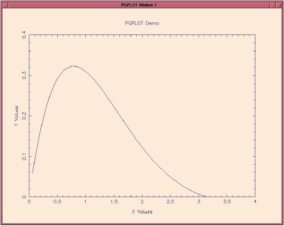
        CALL PGENV(0., 4., 0., .4, 0, 1)
        CALL PGLAB('X Values', 'Y Values', 'PGPLOT Demo')
        CALL PGLINE(100, X, Y)
        CALL PGEND
      DO 20 J=1,5
      PRINT 15, X(J), Y(J)
 15   FORMAT(2X,2F8.3)
 20   CONTINUE
      STOP
      END
      SUBROUTINE TRIG(N,X,Y)
      DIMENSION X(1), Y(1)
      DO 10 I=1,N
      Y(I) = SIN(X(I))*EXP(-X(I))
 10   CONTINUE
      RETURN
      END

Subroutine PGBEN in the pgdemo program performs the plot initialization. Placing the ? character in the PGBEN parameter list causes the program to query for which output device to use. The two calls to PGSCRN simply change the background and foreground colors (and there are plenty colors from which to choose). PGENV establishes the limits of the x- and y-axis, and PGLAB labels the axes and plot. (Math/Greek symbols and subscript/superscript capabilities are available.) The generated curve is plotted by PGLINE, and the plot is completed by PGEND.

This PGPLOT program is compiled by the command:

$ f77 -o pgdemo pgdemo.f -pgplot -lX11

It is necessary to include the X11 library after the PGPLOT library because some of the PGPLOT subroutines create X windows and control their attributes.

Program execution results in the messages shown in Figure 1.

The pgdemo program first queried for which output device to use. I answered with a ? to see the list of available devices (which is configured when the package is installed). From the list I then selected /XWINDOW, and the simple plot shown in Figure 2 was drawn in an X window. PGPLOT supports a long list of output devices, but not all are available for Linux users.

Now the fun can really begin by selecting font sizes, axis types, alphanumeric notations, and a host of other options. If you have had any previous experience with Fortran plotting routines, PGPLOT will be easy to learn and use.

SciLab is one of my favorite programs running under Linux. If you deal with matrix or vector data, signal analysis, nonlinear optimization, plotting, or other mathematical manipulations, you owe it to yourself to explore this feature-packed program. (SciLab was reviewed in Linux Journal, Issue 11, and it is available for a variety of other computer platforms, including Sun Sparc station, IBM RS 6000, HP 9000, DEC Mips, and DEC Alpha.)

Beyond the hundreds of built-in or supplied mathematical functions, SciLab users can also dynamically link their own Fortran and C subroutines to the SciLab binary without recompiling the SciLab source code. The linked subroutines are then available for calling from within SciLab using either interactive commands or by executing scripts.

This important feature allows Fortran users (and C programmers) to make use of “tried and true” source code without the trouble of converting the subroutines to equivalent SciLab macros and scripts that use built-in SciLab functions. Just as important, tedious debugging can be kept to a minimum (provided the linked subroutines have already been tested thoroughly).

Returning once again to our original trivial example code, let's link the subroutine TRIG into a SciLab session. First, we need to compile the TRIG object module using the f77 command:

$ f77 -c trig.f

which produces trig.o in the present working directory. From within Scilab we link trig.o using the link command:

-->link('trig.o','trig')
 linking  "trig_" defined in "trig.o "
 lastlink 0,0

The first argument string in the link command is the name (case sensitive) of the Fortran object module. If this module is not in the current SciLab working directory, you must include the path. The second argument string must be the exact name of the Fortran subroutine being linked; however, case is not important. (Note that SciLab variables are case-sensitive, so subsequent use of trig within SciLab requires that you use lower case.)

Other subroutines also can be linked in the same way, and SciLab lists all linked subroutines when the link command is issued without arguments, i.e.:

-->link()
 ans  =
 trig

Now we are ready to use trig in our SciLab session, but first we need to specify the two input variables (n,x) for the trig subroutine. Below are the commands issued with Scilab echoing the results.

-->n=5
 n  =
    5.
-->x=[.1 .2 .3 .4 .5]
 x  =
!    .1     .2     .3     .4     .5 !

Actually calling trig is done using SciLab's fort command as illustrated below (along with the result) for our example:

-->y=fort('trig',n,1,'i',x,2,'r','out',[1,5],3,'r')
 y  =
! .0903330 .1626567 .2189268 .2610349 .2907863 !

Okay, now for the explanation. On the left-hand side of the entered expression is a list of the subroutine output variables (y in this example). The arguments inside the fort expression consist of three groups. First is the called subroutine name (trig) as a string variable. This is followed by a list of the subroutine input variables, given in this example as:

n,1,'i', x,2,'r'

The first three items are the input variable (n), its position in the trig subroutine argument list (1), and a string character representing the variable's type (i for integer). Likewise, the second input variable is the real array, x, positioned as the second argument in trig. This pattern continues until all the input variables are listed. Variables in the input list do not have to be listed in any particular order. In other words, we could have just as easily listed the inputs as:

x,2,'r', n,1,'i'

Once all the input variables are listed, we can specify the output variable or variables, denoted in this example by:

'out',[1,5],3,'r'

The key word 'out' always appears, followed by a matrix notation informing SciLab that the output variable, y, is a 1x5 array. The 3 gives the position of y in the subroutine's argument list, and r states that the variable is type real.

Subroutines having more than one output variable simply need to list the parameters associated with each variable on the output side in the fort argument list and include each variable on the left-hand side of the expression. For example, assume we have a Fortran subroutine given by:

SUBROUTINE WIN95(IDEAS,BUGS,DOS,DELAY)
REAL*4 BUGS(1,1), DOS, DELAY(1)
INTEGER*2 IDEAS
.
.
.
RETURN
END

The input variables are DOS and IDEAS, and the outputs are BUGS and DELAY. After compiling and linking this subroutine into SciLab, it is called by:

-->bugs,delay]=fort('win95',dos,3,'r',ideas,1,'i',
                 'out'[99,99],2,'r',[1,10],4,'r')

It's as easy as that!

When coupling Fortran subroutines with SciLab, any print statements within your Fortran subroutines will not print to the SciLab session. Instead they print to the X window from which you started SciLab (or on the console monitor if you loaded Scilab from a window manager, such as FVWM). More importantly, the dynamically linked Fortran subroutines can open, read, write, and close disk files. Subroutines containing COMMON blocks must be restructured to accept all the variables and constants through the fort command line.

The Fortran programming language is reasonably well supported in the Linux environment. Furthermore, a variety of high-quality programming tools and libraries provide a capability that, when coupled with all the features of Linux, makes for a potent programming platform for engineers and scientists.

In the future we can expect a robust g77 compiler with debugger support, continued improvement in existing support libraries, and release of new Fortran tools. Perhaps even more exciting is work being done by the Linux-Lab Project. This project is developing drivers to support acquisition of laboratory and field data using Linux. Higher-level interface to most hardware devices will be via C language libraries, which (we hope) will also be callable from our Fortran programs.

So take the plunge, you Fortran fanatics! It will be an exciting adventure!

Thanks to Tony Dalrymple, Rod Sobey, and Gary Howell for helpful comments on this article.