Use Python for Scientific Computing
As computers become more and more powerful, scientific computing is becoming a more important part of fundamental research into how our world works. We can do more now than we could even imagine just a mere decade ago.
Most of this work has been done traditionally in more low-level languages, such as C or FORTRAN. Originally, this was done in order to maximize the efficiency of the code and to squeeze out every last bit of work from the computer. With computers now reaching multi-GHz speeds, this is no longer the bottleneck it once was. Other efficiencies come into play, with programmer efficiency being paramount. With this in mind, other languages are being considered that help make the most of a progammer's time and effort.
This article discusses one of these options: Python. Although Python is an interpreted language and suffers, unjustly, from the stigma that entails, it is growing in popularity among scientists for its clarity of style and the availability of many useful packages. The packages I look at in this article specifically are designed to provide fast, robust mathematical and scientific tools that can run nearly as fast as C or FORTRAN code.
The packages I focus on here are called numpy and scipy. They are both available from the main SciPy site (see Resources). But before we download them, what exactly are numpy and scipy?
numpy is a Python package that provides extended math capabilities. These include new data types, such as long integers of unlimited size and complex numbers. It also provides a new array data type that allows for the construction of vectors and matrices. All the basic operations that can be applied to these new data types also are included. With this we can get quite a bit of scientific work done already.
scipy is a further extension built on top of numpy. This package simplifies a lot of the more-common tasks that need to be handled, including tools such as those used to find the roots of polynomials, doing Fourier transformations, doing numerical integrals and enhanced I/O. With these functions, a user can develop very sophisticated scientific applications in relatively short order.
Now that we know what numpy and scipy are, how do we get them and start using them? Most distributions include both of these packages, making this the easy way to install them. Simply use your distribution's package manager to do the install. For example, in Ubuntu, you would type the following in a terminal window:
sudo apt-get install python-scipy
This installs scipy and all of its dependencies.
If you want to use the latest-and-greatest version and don't want to wait for your distribution to get updated, they are available through Subversion. Simply execute the following:
svn co http://svn.scipy.org/svn/numpy/trunk numpy svn co
http://svn.scipy.org/svn/scipy/trunk scipy
Building and installing is handled by a setup.py script in the source directory. For most people, building and installing simply requires:
python setup.py build
python setup.py install    # done as root
If you don't have root access, or don't want to install into the system package directory, you can install into a different directory using:
python setup.py install --prefix=/path/to/install/dir
Other options also are available, which you can find out about by using:
python setup.py --help-commands
Take time to experiment and see whether you can use any of the extra options in your specific case.
Now that we have scipy and numpy installed, let's begin our tour by looking at some of the basic functions that are often used in scientific calculations. One of the most common tasks is matrix mathematics. This is greatly simplified when you use numpy. The most basic code to do a multiplication of two matrices using numpy would look like this:
import numpy
a1=numpy.empty((500,500))
a2=numpy.empty((500,500))
a3=a1*a2
Contrast this to what we would need to write if we did it in C:
#include <stdlib.h>
int main() {
   double a1[500][500];
   double a2[500][500];
   double a3[500][500];
   int i, j, k;
   for (i=0; i<500; i++) {
      for (j=0; j<500; j++) {
         a3[i][j] = 0;
         for (k=0; k<500; k++) {
            a3[i][j] += a1[i][k] * a2[k][j];
         }
      }
   }
}
The Python code is much shorter and cleaner, and the intent of the code is much clearer. This kind of clarity in the code means that the programmer can focus much more on the algorithm rather than the gritty details of the implementation. There are C libraries, such as LAPACK, which help simplify this work in C. But, even these libraries can't match the simplicity of scipy.
“But what about efficiency?”, I hear you ask. Well, let's take a look at it with some timed runs. Taking our above example, we can put some calls around the actual matrix multiplication part and see how long each one takes. See Table 1 for the results.
Although your mileage will vary, because these times depend on your hardware and what other programs also are running on your machine, we can see a general trend. The Python code actually was about eight times faster than the C code compiled with no command-line options. That is actually quite surprising. Once we use the optimization command-line option, we see that the C code is now faster, by a factor of approximately 25. So, we can get faster code using optimized C, but we need to realize that multiplying two matrices with 250,000 elements each in one-quarter of a second is probably fast enough.
As well, we get a certain amount of protection when we use Python. What happens if we try to multiply two matrices where such multiplication doesn't make sense mathematically? When we try to multiply two matrices of different sizes, Python gives us:
ValueError: shape mismatch: objects cannot be
 broadcast to a single shape
In C, we get no error at all. This due to the fact that when we work with matrices, we actually are using pointer arithmetic. So pretty much anything we do is valid C, even if it makes no sense in the problem domain.
We also can work just as easily with complex numbers. If we wanted to create an array of 64-bit complex numbers, we would write:
a=zeros((500,500), dtype=complex64)
which would give us a 500x500 element matrix initialized with zeros. We access the real and imaginary parts of each element using:
a.real[0,0]=1.0 a.imag[0,0]=2.0
which would set the value 1+2j into the [0,0] element.
There also are functions to give us more complicated results. These include dot products, inner products, outer products, inverses, transposes, traces and so forth. Needless to say, we have a great deal of tools at our disposal to do a fair amount of science already. But is that enough? Of course not.
Now that we can do some math, how do we get some “real” science done? This is where we start using the features of our second package of interest, scipy. With this package, we have quite a few more functions available to do some fairly sophisticated computational science. Let's look at an example of simple data analysis to show what kind of work is possible.
Let's assume you've collected some data and want to see what form this data has, whether there is any periodicity. The following code lets us do that:
import scipy
inFile = file('input.txt', r)
inArray = scipy.io.read_array(inFile)
outArray = fft(inArray)
outFile = file('output.txt', w)
scipy.io.write_array(outFile, outArray)
As you can see, reading in the data is a one-liner. In this example, we use the FFT functions to convert the signal to the frequency domain. This lets us see the spread of frequencies in the data. The equivalent C or FORTRAN code is simply too large to include here.
But, what if we want to look at this data to see whether there is anything interesting? Luckily, there is another package, called matplotlib, which can be used to generate graphics for this very purpose. If we generate a sine wave and pass it through an FFT, we can see what form this data has by graphing it (Figures 1 and 2).
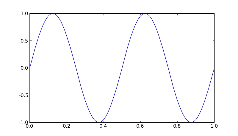
Figure 1. Sine Wave
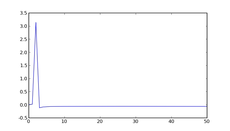
Figure 2. FFT of Sine Wave
We see that the sine wave looks regular, and the FFT confirms this by having a single peak at the frequency of the sine wave. We just did some basic data analysis.
This shows us how easy it is to do fairly sophisticated scientific programming. And, if we use an interactive Python environment, we can do this kind of scientific analysis in an exploratory way, allowing us to experiment on our data in near real time.
Luckily for us, the people at the SciPy Project have thought of this and have given us the program ipython. This also is available at the main SciPy site. ipython has been written to work with scipy, numpy and matplotlib in a very seamless way. To execute it with matplotlib support, type:
ipython -pylab
The interface is a simple ASCII one, as shown in Figure 3.
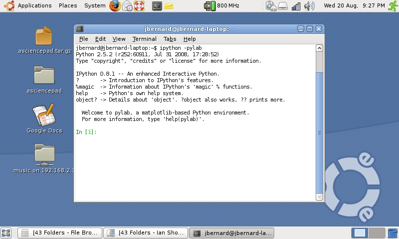
Figure 3. ipython Window
If we use it to plot the sine wave from above, it simply pops up a display window to draw in the plot (Figure 4).
The plot window allows you to save your brilliant graphs and plots, so you can show the entire world your scientific breakthrough. All of the plots for this article actually were generated this way.

Figure 4. ipython Plotting
So, we've started to do some real computational science and some basic data analysis. What do we do next? Why, we go bigger, of course.
So far, we have looked at relatively small data sets and relatively straightforward computations. But, what if we have really large amounts of data, or we have a much more complex analysis we would like to run? We can take advantage of parallelism and run our code on a high-performance computing cluster.
The good people at the SciPy site have written another module called mpi4py. This module provides a Python implementation of the MPI standard. With it, we can write message-passing programs. It does require some work to install, however.
The first step is to install an MPI implementation for your machine (such as MPICH, OpenMPI or LAM). Most distributions have packages for MPI, so that's the easiest way to install it. Then, you can build and install mpi4py the usual way with the following:
python setup.py build python setup.py install
To test it, execute:
mpirun -np 5 python tests/helloworld.py
which will run a five-process Python and run the test script.
Now, we can write our program to divide our large data set among the available processors if that is our bottleneck. Or, if we want to do a large simulation, we can divide the simulation space among all the available processors. Unfortunately, a useful discussion of MPI programming would be another article or two on its own. But, I encourage you to get a good textbook on MPI and do some experimenting yourself.
Although any interpreted language will have a hard time matching the speed of a compiled, optimized language, we have seen that this is not as big a deterrent as it once was. Modern machines run fast enough to more than make up for the overhead of interpretation. This opens up the world of complex applications to using languages like Python.
This article has been able to introduce only the most basic available features. Fortunately, many very good tutorials have been written and are available from the main SciPy site. So, go out and do more science, the Python way.
ScientificPython
numpy and scipy are not the only options available to Python programmers. Another popular package is ScientificPython. It includes geometric types (such as vectors, tensors and quaternions), polynomials, basic statistics, derivatives, interpolation and more. This is the same type of functionality available in scipy. The major difference is that ScientificPython has the ability to do parallel programming built in, whereas scipy requires an extra module. This is done with a partial implementation of MPI and an implementation of the Bulk Synchronous Parallel library (BSPlib).
LAPACK and BLAS
The argument can be made that comparing the complexity of C and FORTRAN to that of Python is unfair, because we actually are using add-on packages in Python. Equivalent libraries can be used in C and FORTRAN, with LAPACK and BLAS being some of the more popular. BLAS provides basic linear algebra functions, while LAPACK builds on these to provide more complex scientific functions. Although these libraries provide optimized routines that will extract every useful cycle from your hardware and are much simpler to write than straight C or FORTRAN, they still are orders of magnitude more complex than the equivalent in Python. If you really do need to squeeze out every last tick from your machine, however, nothing will beat these types of libraries.
Types of Parallel Programming
Parallel programs can, in general, be broken down into two broad categories: shared memory and message passing. In shared-memory parallel programming, the code runs on one physical machine and uses multiple processors. Examples of this type of parallel programming include POSIX threads and OpenMP. This type of parallel code is restricted to the size of the machine that you can build.
To bypass this restriction, you can use message-passing parallel code. In this form, independent execution units communicate by passing messages back and forth. This means they can be on separate machines, as long as they have some means of communication. Examples of this type of parallel programming include MPICH and OpenMPI. Most scientific applications use message passing to achieve parallelism.
Resources
Python Programming Language—Official Web Site: www.python.org
SciPy: www.scipy.org
ScientificPython—Theoretical Biophysics, Molecular Simulation, and Numerically Intensive Computation: dirac.cnrs-orleans.fr/plone/software/scientificpython
Joey Bernard has a background in both physics and computer science. Finally, his latest job with ACEnet has given him the opportunity to use both degrees at the same time, helping researchers do HPC work.