Transform Methods and Image Compression
This article has its origins in a data compression course we've been developing over the past few years at Auburn University. The course is elementary and begins with the basic (text) compression methods of Shannon and Huffman. Some of these methods can be appreciated with pencil-and-paper examples; others, such as images to be modified by compression, need some machine experimentation.
Students may choose to present a project as part of their course evaluation. We've seen various projects, including an amusing example of Huffman-on-a-hand-calculator, an overview presentation of PNG (Portable Network Graphics) and a project concerning smoothing in JPEG.
We will introduce the transform techniques of JPEG and wavelets, discuss some mathematical themes shared by these methods, and illustrate the use of a high-level linear algebra package in understanding such schemes. The images were generated using Octave and Matlab, primarily on GNU/Linux (x86) and Solaris (SPARC), but also on a Macintosh.
Data compression methods with zero information loss have been used on image data for some time. In fact, the popular GIF format uses an LZW scheme (the basic method used in UNIX compress) to compress 256-color images. PNG is more sophisticated and capable, using a predictor (or filter) to prepare the data for a gzip-style compressor. (Greg Roelofs has an introduction to PNG and some notes on patent questions concerning GIF [see Resources 8].) However, applications using high-resolution images with thousands of colors may require more compression than can be achieved with these lossless methods.
Lossy schemes discard some of the data in order to obtain better compression. The problem, of course, is deciding just which information is to be compromised. Loss of information in compressing text is typically unacceptable, although simple schemes such as elimination of every vowel from English text may find application somewhere. The situation is different with images and sound; in those cases, some loss of data may be quite acceptable, even imperceptible.
In the 1980s, the Joint Photographic Experts Group (JPEG) was formed to develop standards for still-image compression. The specification includes both lossless and lossy modes, although the latter is perhaps of the most interest (and is usually what is meant by “JPEG compression”). G. K. Wallace has a paper (see Resources 10) discussing the standard in some detail.
The method in lossy JPEG depends on an important mathematical and physical theme for its compression: local approximation. The JPEG group took this idea and fine-tuned it with results gained from studies on the human visual system. The resulting scheme enjoys wide use, in part because it is an open standard but mostly because it does well on a large class of images, with fairly modest resource requirements.
JPEG and wavelet schemes fall under the general category of transform methods. The development of wavelet techniques has taken place more recently than the classical method in JPEG, and is a consequence of the never-ending search for “better” basic images.
Roughly speaking, the first step in lossy compression schemes like JPEG and wavelets is to break down an image into a weighted sequence of simpler, more basic images. At this stage, the image may be reconstructed exactly from knowledge of the basic images and their corresponding weights. The effectiveness of the method depends to a great extent on the choice of the basic images. Once a set of basic images, or basis, has been chosen, arbitrary images can be replaced by equivalent collections of weights. A basic image having a correspondingly large weight is an indication of its characteristic importance in the overall image. (The assumption here is that the basis images have been normalized, so that they have the same mathematical size.)
The mathematics behind this process is expressed in the language of linear algebra. There is considerable mathematical freedom in the choice of basis images; however, in practice they are usually chosen to exhibit features intrinsic to the class of images of interest. For example, JPEG chooses basic images designed to reflect certain classical spatial frequencies.
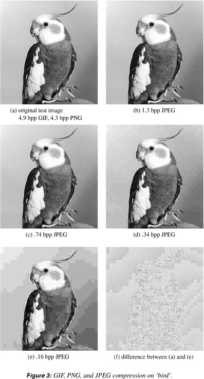
The process of using a basis to resolve an image into a collection of weights is called a transform. To simplify things, we'll consider gray-scale images (color is discussed briefly in the conclusion), which can be represented as mxn arrays of integers. The range of values isn't important in understanding the mathematical ideas, although it is common to restrict values to the interval [0,255], giving a total of 256 levels of gray. As an example, Figure 3(a) shows an image containing 256x256 pixels with 145 shades of gray represented.
Mathematically, any basis for the space of mxn gray-scale images must contain exactly mn images—the number of pixels in an mxn image. Consequently, the transform of an mxn image will have mn weights. The weights can be conveniently arranged into an mxn array called the transformed image even though it isn't a true image at all.
The transformation process, in itself, is certainly not a compression technique (since the transformed image is the same size as the original), but it can lead to one. Suppose the basis images can be chosen so that, for a wide class of images, many of the weights turn out to be small: for a given image, set these small weights to zero and use the resulting array of modified weights to represent it. Since the transform of the image has been modified, it can be used only to approximate the original. How good is the approximation? That depends on how good the scheme is for throwing out nonzero weights, that is, on the appropriateness of the basis elements and the number of weights which can be discarded. JPEG and wavelet methods both employ this type of process and offer significant compression benefits, often with minimal impact on the quality of the reproduction. They differ in the choice of basis images, i.e., in the transform used, and subsequently in the method used to discard small weights. However, both share the idea of picking a basis that can efficiently represent an image, often using only a small number of its basic images.
In this section, several examples using the cosine transform are presented. This transform is used by JPEG, applied to 8x8 portions of an image. An NxN cosine transform exists for every N, which exchanges spatial information for frequency information. For the case N=4, a given 4x4 portion of an image can be written as a linear combination of the 16 basis images which appear in Figure 1(a).

The transform provides the coefficients in the linear combination, allowing approximations or adjustments to the original image based on frequency content. One possibility is simply to eliminate certain frequencies, obtaining a kind of partial sum approximation. The implicit assumption in JPEG, for example, is that the higher-frequency information in an image tends to be of less importance to the eye.
The images in Figure 1 can be obtained from the scripts supplied on our web site (see Resources 4) as follows. We'll use “>” to denote the prompt printed by Matlab or Octave, but this will vary by platform.
Define the test image:
> x = round(rand(4)*50) % 4x4 random matrix,
                       % integer entries in
[0,50]
This will display some (random) matrix, perhaps
    | 10 20 10 41 |
    | 40 30 2  12 |
    | 20 35 20 15 |
and we can view this “image” with the instructions:
> imagesc(x);      % Matlab users
> imagesc(x, 8);   % Octave users
Something similar to the smaller image at the lower left in Figure 1(b) will be displayed. (We chose the 4x4 example for clarity; however, the viewer in Octave may fail to display it properly. In this case, either the image can be padded before display or a larger image can be chosen.) Now ask for the matrix of partial sums (the larger image in Figure 1(b)):
> imagesc(psumgrid(x)); % Display the 16 partial
                        % sums
The partial sums are built up from the basis elements in the order shown in the zigzag sequence above. This path through Figure 1(a) is based on increasing frequency of the basis elements. Roughly speaking, the artificial image in Figure 1(b) is the worst kind as far as JPEG compression is concerned. Since it is random, it will likely have significant high-frequency terms. We can see these by performing the discrete cosine transform:
> Tx = dct(x, 4) % 4
                 % of x
For the example above, this gives the matrix
     | 79.25   9.47  4.75 -11.77 |
     |  6.25 -19.69 -4.25 -11.60 |
     |  5.97   8.02 12.73 -15.64 |
of coefficients used to build the partial sums in Figure 1 from the basis elements. The top left entry gets special recognition as the DC coefficient, representing the average gray level; the others are the AC coefficients, AC0,1 through AC3,3.
The terms in the lower right of Tx correspond to the high-frequency portion of the image. Notice that even in this “worst case”, Figure 1 suggests that a fairly good image can be obtained without using all 16 terms.

The process of approximation by partial sums is applied to a “real” image in Figure 2, where 1/4, 1/2 and 3/4 of the 1024 terms for a 32x32 image are displayed. These can be generated with calls of the form:
> x = getpgm('math4.pgm'); % Get a graymap image
> n = length(x);        % n is the number of rows
                        % in the square image
> y = psum(x, n*n / 2); % y is the partial sum
                        % using 1/2 of the terms
> imagesc(y);           % Display the result
Our approximations retain all of the frequency information corresponding to terms from the zigzag sequence below some selected threshold value; the remaining higher-frequency information is discarded. Although this can be considered a special case of a JPEG-like scheme, JPEG allows more sophisticated use of the frequency information.
JPEG exploits the idea of local approximation for its compression: 8x8 portions of the complete image are transformed using the cosine transform, then each block is quantized by a method which tends to suppress higher-frequency elements and reduce the number of bits required for each term. To “recover” the image, a dequantizing step is used, followed by an inverse transform. (We've ignored the portion of JPEG which does lossless compression on the output of the quantizer, but this doesn't affect the image quality.) The matrix operations can be diagrammed as:
  transform    quantize     dequantize     invert
x  ------>  Tx  ----->  QTx  -------> Ty  ---> y
In Octave or Matlab, the individual steps can be written:
> x = getpgm('bird.pgm'); % Get a graymap image
> Tx = dct(x);       % Do the 8
> QTx = quant(Tx);   % Quantize, using standard
                     % 8
> Ty = dequant(QTx); % Dequantize
> y = invdct(Ty);    % Recover the image
> imagesc(y);        % Display the image
To be precise, a rounding procedure should be done on the matrix y. In addition, we have ignored the zero-shift specified in the standard, which affects the quantized DC coefficients.
It should be emphasized that we cannot recover the image completely—there has been loss of information at the quantizing stage. It is illustrative to compare the matrices x and y, and the difference image x-y for this kind of experiment appears in Figure 3(f). There is considerable interest in measuring the “loss of image quality” using some function of these matrices. This is a difficult problem given the complexity of the human visual system.
The images in Figure 3 were generated at several “quality” levels, using software from the Independent JPEG Group (see Resources 5). The sizes are given in bits per pixel (bpp); i.e., the number of bits, on average, required to store each of the numbers in the matrix representation of the image. The sizes for the GIF and PNG versions are included for reference. (“Bird” is part of a proposed collection of standard images at the Waterloo BragZone [see Resources 11] and has been modified for the purposes of this article.)
One troublesome aspect of JPEG-like schemes is the appearance of “blocking artifacts,” the telltale discontinuities between blocks which often follow aggressive quantizing. The image on the left in Figure 6 was produced using a scalar multiple of the suggested luminance quantizer. Clearly visible blocks can be seen, especially in the “smoother” areas of the image.
JPEG operates on individual 8x8 blocks in the image and processes them independently. There can be significant loss of detail information within the individual blocks if the quantizing is aggressive. The cosine transform used in JPEG has properties which may (indirectly) help smooth the transition between neighboring blocks; however, the tracks of the block-by-block processing can be apparent when the blocks are reassembled and the image restored. In this case, it may be desirable to implement a smoothing scheme as part of the restoration process. This section considers the back-end smoothing procedure discussed in the book JPEG Still Image Data Compression Standard (see Resources 7).
The JPEG decompresser may have only rough estimates about much of the original frequency information, but it typically has fairly good estimates of the average level of gray in each original 8x8 block (because of the way quantizers are chosen). The idea is to use the average gray (DC-coefficient) information of its nearest neighbors to adjust a given block's (AC-coefficient) frequency information. Figure 4 illustrates the process with a single “superblock” consisting of a center 8x8 image and its nearest neighbors. The center block in the image on the right has been “smoothed” by the influence of its nearest neighbors (the surrounding eight 8x8 blocks).

The process on a more complicated image is illustrated in Figure 5. Here, the image is plotted as a surface where, at each pixel (y,x), the height of the surface represents the gray value. For a given 8x8 block, the 3x3 superblock consisting of its nearest neighbors contains 3282 total entries. The polynomial
+ a6y2 + a7x + a8y + a9
is fitted by requiring that the average value over each subblock matches the average gray estimate (this gives nine equations for the unknowns a1,...,a9). The polynomial defines a surface over the center block, which approximates the corresponding portion of the original surface. Figure 5 shows a surface in (a) and its polynomial approximation in (b).

The JPEG decompresser can perform the transform procedure on a polynomial approximation, obtaining a set of predictors for the frequency information of the original image. The original estimates passed by the compressor can be adjusted using these predictors in the hope of reducing the blocking problem.
In Figure 5, the lowest five frequencies were considered for adjustment by the predictors: zero values passed by the compressor were replaced by the predicted values (subject to a certain clamping). The procedure applied to an aggressively-quantized bird image appears in Figure 6. The deblock.m script (see Resources 4) performs the smoothing. The following code was used to generate the right-hand image:
> x = getpgm('bird.pgm'); % Get a graymap image
> Tx = dct(x);       % Do the 8
> QTx = quant(Tx, 4*stdQ); % Quantize, using
                           % 4*luminance
> Ty = dequant(QTx);       % Dequantize
> Tz = deblock(Ty);        % Smooth
> z = invdct(Tz);          % Recover the image
> imagesc(z);              % Display the image

This kind of smoothing scheme is attractive, in part because of its simplicity and the fact that it can be used as a back-end procedure to JPEG (regardless of whether the original file was compressed with this in mind). However, JPEG achieves its rather impressive compression by discarding information. The smoothing procedure sometimes makes good guesses about the missing data, but it cannot recover the original information.
Features of a signal we wish to examine can guide us in our quest for the “right” basis vectors. For example, the cosine transform is an offspring of the Fourier transform, the development of which was, in a sense, a consequence of the search for basic frequencies with which periodic signals could be resolved.
The Fourier transform is an indispensable tool in the realm of signal analysis. When used as a compression device, we might wish it had the additional capacity of being able to highlight local frequency information—generally, it doesn't. The weights given by the Fourier expansion of a signal may yield information about the overall strength of the frequencies, but the information is global. Even if a weight is substantial, it doesn't normally give us any clue as to the location of the “time interval” over which the corresponding frequency is significant.
The interest in and use of wavelet transforms has grown appreciably in recent years since Ingrid Daubechies (see Resources 1) demonstrated the existence of continuous (and smoother) wavelets with compact support. They have found homes as theoretical devices in mathematics and physics and as practical tools applied to a myriad of areas, including the analysis of surfaces, image editing and querying and, of course, image compression.
In this section, we present an example using the Haar wavelet, which in one sense is the simplest of wavelets. The 16 basis elements in Figure 7 form a basis for the set of 4x4 images. Compare these with the cosine transform elements in Figure 1. One can begin to see the formation of elements with localized supports even at this “coarse” resolution level.

The simple (lossy) compression scheme used in the example is not as elaborate as the quantizing scheme used in JPEG. Basically, we throw away any weight which is smaller than some selected threshold value. In Figure 8, we have used this simple scheme on “bird” at several tolerance settings.
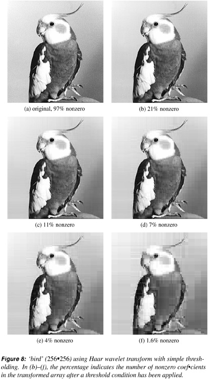
Setting a weight to zero in the transformed image is equivalent to eliminating the corresponding basis array in the expansion of the image. This illustrates a certain kind of simple-minded partial sum (projection) approach to compression, similar to the example in Figure 2. Examples of more sophisticated wavelet schemes can be done with Geoff Davis' Wavelet Image Compression Construction Kit (see Resources 2). Strang's article (see Resources 9) provides a short, elementary introduction to wavelets.
The discussion of JPEG and wavelets has centered on gray-scale images. Color images may assign a red, green and blue triple (rgb) to each pixel, although other choices are possible. Color specified in terms of brightness, hue and saturation, known as luminance-chrominance representations, may be desirable from a compression viewpoint, since the human visual system is more sensitive to errors in the luminance component than in chrominance (see Resources 7). Given a color representation, JPEG and wavelet schemes can be applied to each of the three planes.
This article was adapted from a recent book (see Resources 3). More information, such as details of the smoothing procedure, along with the scripts and complete documentation may be obtained from our web site (see Resources 4).
Information on Matlab (for GNU/Linux and other platforms) is available through http://www.mathworks.com/. Octave is developed by John W. Eaton with contributions from many folks, and is distributed under the GNU General Public License. Complete sources and ready-to-run executables for several platforms are available via anonymous ftp from ftp.che.wisc.edu in the /octave directory. An introduction to Octave appeared in a previous Linux Journal article (see Resources 6) and on-line information can be found via http://www.che.wisc.edu/octave/.

Darrel Hankerson joined the faculty at Auburn University after completing a degree in mathematics at the University of Utah. Along with Greg A. Harris and Peter D. Johnson, Jr., he is the author of Introduction to Information Theory and Data Compression, CRC Press, 1997.