Linux is a virtually unparalleled platform for using freely distributable software. The kernel source is free, the standard utilities are free and so is the X Window System. The whole concept of using free software is incredibly appealing, and many users are tempted to try running their systems without any commercial products whatsoever. Yet this desire is often thwarted by a single missing application; desktop publishing and presentation software are commonly cited as current “holes” in the Linux arsenal.

I was faced with such a problem when I decided to abandon the MS-DOS partition on my hard drive and go all Linux. Since I work with a fair amount of statistical information, I needed a straightforward way to summarize data, plot it and perform regression as needed. gnuplot is great for plotting, but that's all it does. Octave and MuPad have powerful numerical features, but they are overkill for simple statistical chores. Unable to find a program that fit this niche, I decided to write one. The result is xldlas, a program for statistics. In the grand Unix tradition, its name is a pseudo-acronym which stands for “x lies, damned lies, and statistics.” The first public release in October 1996 met with quite positive feedback from users, and one of those beta testers (Hans Zoebelein) suggested an article in Linux Journal might be a good way to introduce xldlas to a wider audience. The people at LJ agreed, and asked me to write this overview. The program runs under the X Window System, and is built using the XForms library. You'll find information on how to download xldlas and associated software at the end of this article.

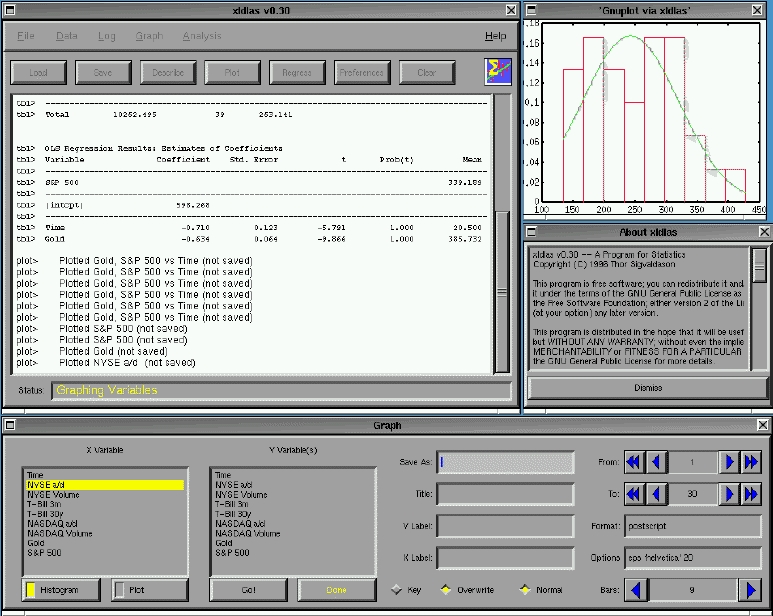
The philosophy behind xldlas is to offer standard statistical tools via an easy-to-use point and click interface. To facilitate this approach, common commands are grouped together into a set of menus. In addition, frequently used commands are available via buttons (See Figure 1).

Figure 1: The xldlas User Interface

Like most statistics packages, xldlas handles a random variable as a vector of values. So a single variable name can refer to dozens, hundreds or thousands of observations.* By grouping data points together under variable names, it is easy to perform relatively complex operations by selecting a few variables and clicking on the relevant command.

*By default, xldlas has a limit of 100 variables of 10,000 observations each. These constraints can easily be adjusted by changing the values for MAX_VARS and MAX_OBS in the source code file xldlas.h.

Of course, before you can perform any kind of statistical operations, you have to get data into xldlas. Since ASCII is the de facto standard for exchanging information under Linux, xldlas allows you to read in space-delimited data from a text file by using the Import command. You supply a file name, and tell xldlas whether the data is in column or row format. The import routine automatically figures out how many variables and observations there are, and reads in the data. To take a concrete example, suppose you have a file which contains space-delimited data on rainfall, temperature and barometric pressure for a single location. After importing this file, xldlas will have three variables in memory, which will be called unknown0, unknown1 and unknown2. You can change these names to anything you like using the Rename command, which is accessible from the Data menu. In addition to this simple ASCII format, xldlas can read and write sets of data in its own proprietary file format. By convention, these files have an .lda extension. Since variable names, descriptions and other useful information are stored in these files, it's generally a good idea to save all your data this way if you plan on using xldlas frequently. The Load, Save and Import commands can all be found in the File menu. To input data by hand, erase variables or perform any kind of editing, there are a number of related commands grouped together in the Data menu. Of these, the most frequently used is probably the Describe command, which generates a table in the main xldlas window showing you the name, number of observations, and a description of every variable currently in memory. In addition to changing observation values, the Edit command can also be used to enter a description for a variable.

Another frequently used item in the Data menu is the Generate command. This routine allows you to perform mathematical transformations on existing data. To continue with the weather example from above, suppose we want to convert our rainfall variable from millimeters to centimeters. With a few clicks of the mouse, we can easily accomplish this task. We could also add some random noise, find the log of the data, or what have you. It's a far cry from Mathematica, but for simple operations the Generate command is quick and easy to use.

Once you have your data loaded, edited and transformed, the next logical step is to perform some kind of statistical work on it. To get a tabular summary of a single variable, including mean, variance, skewness and kurtosis, there's the Summarize command. If you want to check multiple variables for linear relationships, the Correlation command will produce a table of Pearson coefficients. Similarly, the ANOVA command lets you perform one-way and two-way analyses of variance by simply selecting variable names with your mouse and clicking the Go button.

The workhorse of statistical techniques, ordinary least squares regression, is available via the Regress command. Just select a single variable from the dependent browser, any number from the independent browser, and press Go. If you want to store fitted values, then you can enter a new variable name in the regression window. The output of the regression command is a set of three tables, which summarize the fit of the regression, break down the sum of squares deviations and list coefficient estimates. Relevant t-statistics and their associated probabilities are automatically included, as is the F coefficient and confidence level for a joint test of all the estimates.

xldlas also offers two experimental data fitting routines that use connectionist artificial intelligence techniques. The first, GA Fit, uses genetic algorithms to build a fit equation that minimizes the sum of squares between fitted values and actual observations of a given dependent variable. The second, NN Fit, creates a back-propagation neural network using selected independent variables for the input layer, and a single dependent variable for the output layer. In both cases, the fitted values from these techniques can be stored under a supplied variable name. These routines are sometimes useful for exploring non-linear relationships in data that are generally difficult to examine using standard OLS regression.*

*Although not part of the “standard” statistical toolkit, these sorts of AI techniques are becoming increasingly common in various contexts and are great for data mining. Although their implementations in xldlas are fairly rudimentary, more sophisticated modifications are likely if users request them.

In addition to manipulating data and performing analysis, xldlas allows you to graph variables. All of xldlas's graphical output is actually performed by gnuplot, an application which is included in all major Linux distributions. Two graphing commands are implemented: Plot and Histogram. The former lets you create line and scatter plots, while the latter generates a histogram describing a variable's distribution. Both sorts of graphs can be titled and labeled, and they can be saved in any format supported by whatever version of gnuplot is installed on your system. In addition, you can set point and line styles, and the Histogram routine includes an optional feature which will superimpose a normal distribution with the same mean and variance as the data being graphed.

xldlas also provides fairly powerful logging facilities. The Log command allows you to echo all of xldlas's output to an ASCII file. A more powerful tool is the TeXLog command, which allows you to create a PlainTeX format log file with a user-supplied name. All subsequent output, such as regression tables, is written to this file in TeX format. Under xldlas's default configuration, all saved graphs are also included as Encapsulated PostScript insertions. This makes writing statistical papers (such as homework assignments) quite fast and efficient, since much of the time-consuming TeX markup is done automatically.

Finally, all xldlas commands are documented on-line in the Help menu. There are also a number of on-line tutorials, which many users of xldlas have found to be a very useful introduction.

There are currently plans afoot to add a number of features to xldlas. Regressions using Probit and Logit models are high on the to-do list. A set of statistical filters is also likely to be available before long, making it possible to easily detrend data, remove outliers, and so on. HTML format log files will soon be supported. Another important task is to expand the documentation in the source code so it can be more easily modified by people other than the original author.

Like almost all freely distributable software, xldlas development is driven by user feedback. If there are features you want to see, send me some e-mail, preferably with a reference to the algorithm you would like to see implemented.

The best way to get a copy of xldlas is from its homepage at www.a42.com/~thor/xldlas. If you only have FTP access to the Internet, you can get it from ftp://sunsite.unc.edu/ (in pub/Linux/X11/xapps/math/). Both full source and a Linux ELF executable are included in the distribution, which is named xldlas-X.Y-srcbin.tgz, where X.Y is the version number (0.40 at the time of writing).

To run the included executable or compile from the source code, you'll need to have the XForms library installed on your system. For more information about XForms, visit the XForms homepage at bragg.phys.uwm.edu/xforms. Although designed to run under Linux, xldlas will apparently compile under almost all flavours of Unix for which the Xforms library exists, although a little tinkering with the Makefile is sometimes necessary. Make sure you look at the README file included in every distribution to get the latest news on compiling and running xldlas.

gnuplot is available at sunsite.unc.edu/pub/Linux/apps/math/gplotbin.tgz. It is also included in most Linux distributions.

For full functionality, xldlas also requires you to have a fairly complete TeX package installed on your machine. NTeX and teTeX are commonly used under Linux, and are available at http://sunsite.unc.edu/pub/Linux/apps/tex/.