
UpFront
UpFront
- BackupPC
- diff -u: What's New in Kernel Development
- Non-Linux FOSS
- Linux for Science
- Pithos
- Snowy—If Ubuntu One Leaves You Feeling Cold
- They Said It
- LinuxJournal.com—a Fantastic Sysadmin Resource
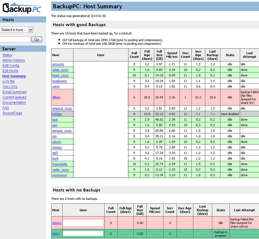
BackupPC
Some tools are so amazing, but unfortunately, if no one ever talks about them, many folks never hear of them. One of those programs is BackupPC. You may have heard Kyle Rankin and myself talk about BackupPC on the Linux Journal Insider podcast, or perhaps you've seen us write about it here in Linux Journal before. If you haven't checked it out, you owe it to yourself to do so. BackupPC has some great features:
Hard drive-based backups, no tape swapping.
Support for NFS, SSH, SMB and rsync.
Hard linking to save valuable disk space.
Individual files can be restored in place in real time.
Powerful and simple Web interface.
E-mail notification on errors.
Free!
BackupPC is one of those projects that doesn't get updated terribly often. It doesn't have flashy graphics. It doesn't require constant maintenance. It just works, and it works well. Check it out: backuppc.sourceforge.net.
diff -u: What's New in Kernel Development
In the ongoing saga of big-kernel-lock removal, we seem to be getting very, very close to having no more BKL. Its remaining users in the linux-next tree seem to be down to less than 20, and most of those are in old code that has no current maintainer to take care of it. Filesystem code, networking code and a couple drivers are all that remain of the once ubiquitous big kernel lock. Arnd Bergmann has posted a complete list of offending code, and a large group of developers have piled on top of it.
The truly brilliant part of ditching the BKL is that a lot of people felt completely stymied by it for a long time. It was absolutely everywhere, and there didn't seem to be any viable alternative. Then the wonderful decision was made to push all the occurrences of the big kernel lock out to the periphery of the kernel—in other words, out to where only one thing would depend on any particular instance. Before that decision, the BKL was deep in the interior, where any given instance of it would be relied on by whole regions of code, each relying on different aspects of it. By pushing it out to the periphery, all of a sudden it became clear which features of the BKL were actually necessary for which of its various users.
As it turned out, most BKL users could make do with a much simpler locking structure, although a few had more complex needs. But, that whole period of time is really cool, because the problem went from being super-intractable, to being pretty well tractable, and by now, it's almost tracted right out of existence.
If you do any kernel development, you'll notice the LKML-Reference tag in every git patch submission, but it might not make total sense to you in this age of on-line e-mail clients, if you haven't read www.faqs.org/rfcs/rfc5322.html lately. Recently, it came up on linux-kernel, that maybe the LKML-Reference tag should just be a URL linking to the linux-kernel post corresponding to that git submission, as stored in any one of many linux-kernel Web archives. But, as several folks pointed out at the time, URLs come and go. Message-ID headers are eternal.
In the old days, the question of which GCC version to support was largely a question of which GCC version managed to piss off Linus Torvalds. Back then, the question tended to be, “How long can we keep compiling with this extremely old version of GCC, now that the GCC developers have implemented this weird behavior we don't like?” Nowadays, the question is more along the lines of, “How soon can we stop supporting kernel compilations under this very old version of GCC that is quirky and requires us to maintain weird stuff in the kernel?”
The question came up recently of whether it would be okay to stop supporting the 3.3 and 3.4 versions of GCC. It turns out that even though GCC 3.3.3 has problems that make it not work right with the latest kernels, certain distributions ship with a patched version that they also call GCC 3.3.3. So, any attempt to alert users to the potential breakage would cause only further confusion. Meanwhile, GCC 3.4 apparently is being used by most embedded systems developers, for whatever reason. And, GCC 3.4 also is a lot faster on ARM architectures than more recent versions of GCC are. So for the moment at least, it seems that those are the oldest versions of GCC still supported for kernel compiling. You also can use more recent GCC versions if you like.
Non-Linux FOSS
There may be a battle in the Linux world regarding what instant-messaging client is the best (Pidgin or Empathy), but in the OS X world, the battle never really started. Adium is an OS X-native, open-source application based on the libpurple library. Although there is a native Pidgin client for OS X, it's not nearly as polished and stable as Adium. With Apple's reputation for solid, elegant programs, the Open Source community really showed it up with this answer to Apple's iChat program. Adium wins on multiple levels, and its source code is as close as a click away. If you ever use OS X and want to try some quality open-source goodness running on the “other” proprietary operating system, check out Adium: www.adium.im.

Linux for Science
Welcome to a new series of short articles on using Linux and open-source software for science. The tools available for free (as in beer) have lowered the cost of participating in computational science. The freedom (as in speech) you have when using these tools allows you to build upon the work of others, advancing the level of knowledge for everyone.
In this series, I'll look at some small science experiments anyone can do at home, and then consider some tool or other available on Linux that you can use to analyze the results. In some purely theoretical spheres (like quantum chemistry or general relativity), I'll just look at the tool alone and how to use it without the benefit of an accompanying experiment.
The first experiment is a classic—the simple pendulum (en.wikipedia.org/wiki/Pendulum). When you look at a simple pendulum, there are two obvious parameters you can change: the mass of the pendulum bob and the length of the string. A simple way to do this at home is to use a bolt with nuts. You can tie a string to the head of a bolt and tie the other end to a pivot point, like a shower-curtain rod. Then, you simply can add more weight by adding nuts to the bolt. This is the basic experimental setup for this article.
The data to collect is the time it takes for each oscillation (one full back-and-forth motion). Because you will want to figure out which parameters affect the pendulum, you'll need to do this for several different masses and lengths. To help get consistent times, let's actually time how long it takes for ten oscillations. To average out any reaction time issues in the time taking, let's do three of these measurements and take the average. You should end up with something like Table 1.
Table 1. Pendulum Data
| Length (cm) | Weight (g) | Time (s) |
|---|---|---|
| 18.8 | 102.0 | 0.9 |
| 18.8 | 118.5 | 0.9 |
| 18.8 | 135.0 | 0.9 |
| 18.8 | 151.5 | 0.9 |
| 37.6 | 102.0 | 1.3 |
| 37.6 | 118.5 | 1.3 |
| 37.6 | 135.0 | 1.3 |
| 37.6 | 151.5 | 1.3 |
| 57.6 | 102.0 | 1.5 |
| 57.6 | 118.5 | 1.5 |
| 57.6 | 135.0 | 1.5 |
| 57.6 | 151.5 | 1.5 |
| 88.8 | 102.0 | 1.9 |
| 88.8 | 118.5 | 1.9 |
| 88.8 | 135.0 | 1.9 |
| 88.8 | 151.5 | 1.9 |
Now that you have the data, what can you learn from it? To do some basic analysis, let's look at Scilab (www.scilab.org). This is a MATLAB-like application that can be used for data analysis and graphing. Installing on Ubuntu, or other Debian-based distributions, is as simple as:
sudo apt-get install scilab
On startup, you should see something like Figure 1.
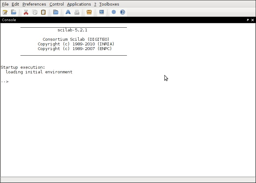
Figure 1. Scilab Startup
Usually, the first thing you'll want to do is graph your data to see whether any correlations jump out at you. To do that, you need to get your data into Scilab. The most natural format is three vectors (length, mass and time), with one row for each measurement you made. In Scilab, this would look like the following:
height = [18.8, 18.8, 18.8, 18.8,
          37.6, 37.6, 37.6, 37.6,
          57.6, 57.6, 57.6, 57.6,
          88.8, 88.8, 88.8, 88.8];
weight = [102.0, 118.5, 135.0, 151.5,
          102.0, 118.5, 135.0, 151.5,
          102.0, 118.5, 135.0, 151.5,
          102.0, 118.5, 135.0, 151.5];
times = [0.9, 0.9, 0.9, 0.9,
         1.3, 1.3, 1.3, 1.3,
         1.5, 1.5, 1.5, 1.5,
         1.9, 1.9, 1.9, 1.9];
You probably will want to use this data over and over again, doing different types of analysis. To do this most simply, you can store these lines in a separate file and load it into your Scilab environment when you want to use it. You just need to call exec() to load and run these variable assignments. For this example, load the data with:
exec("~/pendulum1.sce");
You can see individual elements of this data using the disp() function. To see the first value in the times vector, you would use what's shown in Figure 2. To do a simple 2-D plot, say, of height vs. times, simply execute:
plot(height, times);
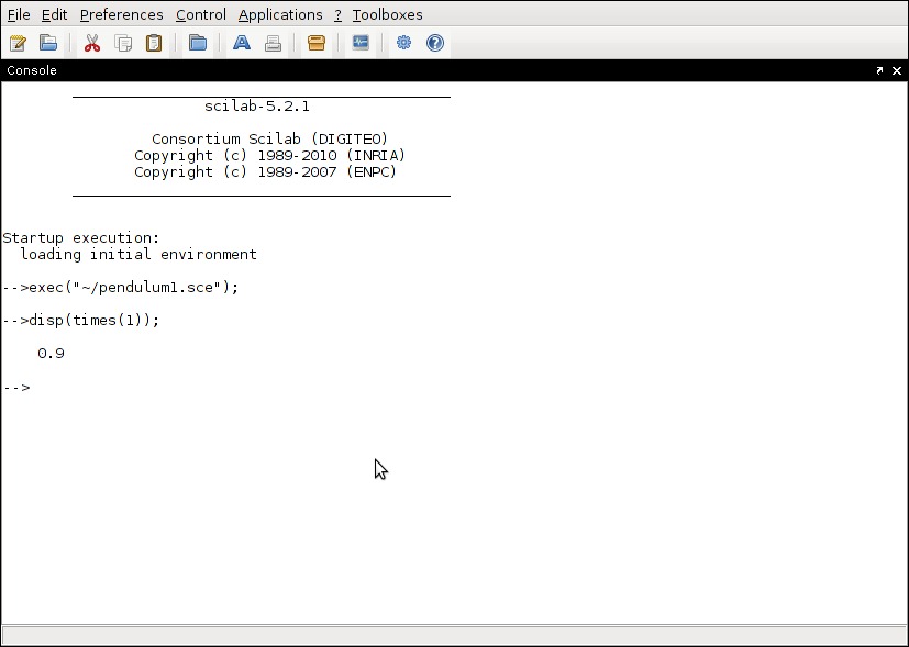
Figure 2. First Value in the Times Vector
This doesn't look very descriptive, so let's add some text to explain what this graph shows. You can set labels and titles for your graph with the xtitle command:
xtitle("Pendulum Height vs Time", "Height(cm)", Time(s)");
This produces a graph that looks like Figure 3. But, you have three pieces of data, or three dimensions. If you want to produce a 3-D graph, use:
surf(height, weight, times);
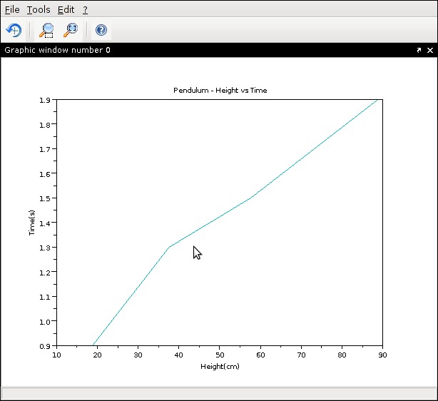
Figure 3. Pendulum Height vs. Time
This produces a surface plot of the data. Because this experiment seems so clear, you won't actually need a full 3-D plot.
All of this data visualization points to weight not really having any influence on time. So, let's focus on the relationship between the length of the pendulum and the time. The graph looks like an almost straight line, so let's assume that it is and see where we get with it. The formula for a straight line is y=a+bx. The typical thing to do is to try to fit a “closest” straight line to the data you have. The term for this is linear regression. Luckily, Scilab has a function for this called regress(). In this case, simply execute:
coeffs = regress(height, times);
disp(coeffs(1));
disp(coeffs(2));
This ends up looking like Figure 4. From this, you can see that the slope of the straight line you just fit to your data is 0.0137626 s/cm. Does this make sense? Let's look at some theory to check out that number.

Figure 4. Using Scilab's regress() Function
According to theory, you should have plotted the square of the time values against the length of the pendulum. To get the square of the time values, use:
timess = times .* times;
This multiplies the first entry of the time vector to itself, the second entry to itself (and so on), down the entire vector. So, the new vector timess contains the square of each entry in the vector times. If you now do a linear regression with timess instead of times, you get the following result:
a = 0.1081958
b = 0.0390888
According to theory, the value of a should be given by ((2 * PI)2 / g), where g is the acceleration due to gravity. According to Scilab, the value is:
ans = (2 * 3.14159)^2 / (9.81 * 100);
disp(ans);
You need to adjust the value of g by a factor of 100 to change it to the correct units of cm, and this gives you 0.0402430. To the second decimal place, this gives you 0.04 from the experiment and 0.04 from theory. What does this look like graphically? You can generate the two graphs with:
plot(height, timess);
plot(height, 0.1081958 + 0.0390888*height);
xtitle("Simple Pendulum", "Length (cm)", "Times Squared (s^2)");
This looks like Figure 5. It seems like a reasonably close match, considering that the spread of measured pendulum lengths covers only 70cm. If you made measurements with pendulum lengths over a larger range of values, you likely will see an even closer match to theory. But, as an easy example experiment to show a small list of Scilab functions, you've already seen that simple pendulums seem to follow theory reasonably well.
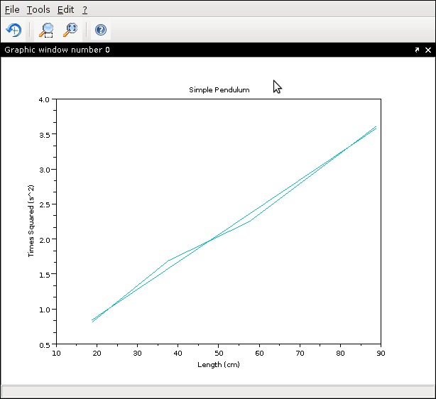
Figure 5. Simple Pendulum Graph
Next month, I'll introduce Maxima and take a look at the math behind the theory of the simple pendulum, seeing whether I can derive the usual results as taught in introductory physics.
If you want me to cover any specific areas of computational science, please contact me with your ideas.
Pithos
I love Pandora Radio. I really do. Unfortunately, the Web browser is an awkward interface for listening. Oh sure, it's effective and works fine. But, it's missing things like media key support, and if you accidentally close your browser window, BOOM—no music.
Enter Pithos. With a very simplistic interface, Pithos doesn't do much, but what it does, it does very well—plays Pandora Radio. If your keyboard has multimedia keys, you'll appreciate Pithos' media key support as well. If your phone rings, simply press the pause button on your keyboard to pause the music regardless of whether the application has focus.
If you like Pandora Radio, check out Pithos. It's worth the download: kevinmehall.net/p/pithos.

Snowy—If Ubuntu One Leaves You Feeling Cold
Canonical has quite a cloud service going with Ubuntu One. It syncs files, music, preferences, contacts and many more things. But, it's only partially free, and the server is completely private and proprietary. The philosophy of keeping the server bits completely closed turns off many of us in the Open Source community. Yes, Canonical has every right to develop Ubuntu One as it sees fit, but as users, we also have the right to look elsewhere. Enter Snowy. No, it's not an all-encompassing replacement for Ubuntu One, but Snowy is designed as a free (in both senses) syncing solution for Tomboy Notes.
If you want to access your Tomboy Notes on-line as well as from several computers while keeping them all in sync, keep your eye on Snowy. The developers hope to get a free syncing service on-line, powered by Snowy, by the time Gnome 3.0 launches. Of course, you also can download Snowy yourself and host your notes on your own server, which is exactly what we hoped Ubuntu One would be when we first heard about it. Check out the progress at live.gnome.org/Snowy.

They Said It
Never underestimate the determination of a kid who is time rich and cash poor.
—Cory Doctorow, Little Brother, 2008
For a list of all the ways technology has failed to improve the quality of life, please press three.
—Alice Kahn
Technology adds nothing to art.
—Penn Jillette, WIRED magazine, 1993
Technology...the knack of so arranging the world that we don't have to experience it.
—Max Frisch
Imagine if every Thursday your shoes exploded if you tied them the usual way. This happens to us all the time with computers, and nobody thinks of complaining.
—Jef Raskin, interviewed in Doctor Dobb's Journal
If computers get too powerful, we can organize them into a committee—that will do them in.
—Bradley's Bromide
LinuxJournal.com—a Fantastic Sysadmin Resource
As you flip though the pages of this month's Linux Journal, you will find a wealth of resources to help you with a variety of system administration tasks. When you have thoroughly absorbed it all, and your head is in danger of exploding, I'd like to offer you an additional resource that will help you achieve total sysadmin Nirvana—LinuxJournal.com. Visit www.linuxjournal.com/tag/sysadmin to find a constant flow of tips and tricks, industry commentary and news. You'll stay up to date on trends and discover new tools to add to your bag of tricks with the help of LinuxJournal.com.
If you are a Linux sysadmin, slap a bookmark on that page and visit often. Please also consider leaving a comment while you're there. We'd like to hear your feedback, as well as have the opportunity to interact with you, our readers. Best of all, you can contribute your own tips, tricks and hacks. Just e-mail webeditor@linuxjournal.com if you have something to share, and you could be published at LinuxJournal.com. We look forward to hearing from you!
