Parallel Programming with NVIDIA CUDA
Programmers have been interested in leveraging the highly parallel processing power of video cards to speed up applications that are not graphic in nature for a long time. Here, I explain how to do this with the CUDA API from NVIDIA. If your GPU is not from NVIDIA, you are not out of luck, as the same can be achieved with other APIs, such as the ATI-based Stream SDK or OpenCL.
With GPGPU, general-purpose applications are executed directly on the streaming processors of video cards. Under the stream processing paradigm, a data set is named a stream. You can think of it much like “file streams” provided by an OS's pipe function.
Streams can be any isolated piece of data, such as a stream of business events or a set of scientific data. Parallel operations are applied on streams with operators, such as split, compute or merge. Figure 1 shows several streams of data and compute operators in parallel.
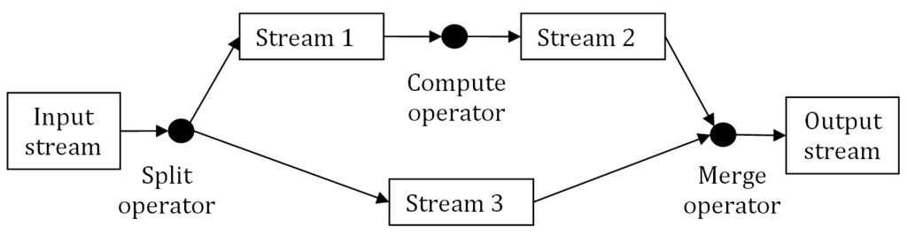
Figure 1. Stream Processing Diagram
Stream processing has been used successfully for general programming, including dataflow programming, financial calculation and industrial automation, just to name a few. Furthermore, system engineers and vendors such as Dell, ASUS, Western Scientific and Microway are building clusters of video cards that are similar to supercomputers, and they're available at a fraction of the cost of their CPU-based counterparts.
You can find many examples of real-life applications that were sped up using CUDA acceleration showcased by NVIDIA at www.nvidia.com/cuda.
Now that I've brushed upon what CUDA and stream processing are, let's start looking into a couple compute-intensive algorithms you can use to give it a spin.
Vector fields are constructs employed in a variety of professions. In robotics, vector fields can help a mobile robot navigate through a room. Let's define a destination and add one or more obstacles. A good scenario for testing CUDA consists in calculating a series of vectors that indicate the direction a robot should follow in order to reach its destination while avoiding all the obstacles present. The robot should also avoid local minima (see below). Figure 2 shows the robot and vector field (the green arrows are the “vectors”).
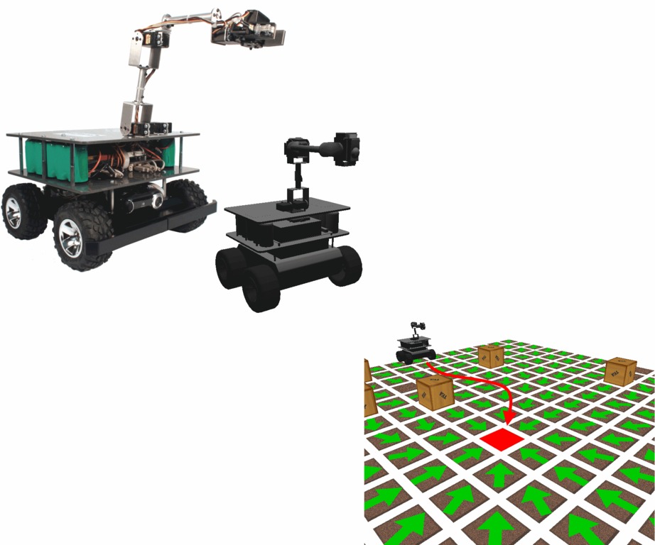
Figure 2. The mobile robot wants to reach the center of the board. The vector field shows the way.
I refer to the target point as an attractor and to obstacles as repulsors—the arrows point toward the attractor and away from repulsors (Figure 3). So, how do you calculate the vector field? The vector field is composed of a series of individual fields, one for each attractor and repulsor.
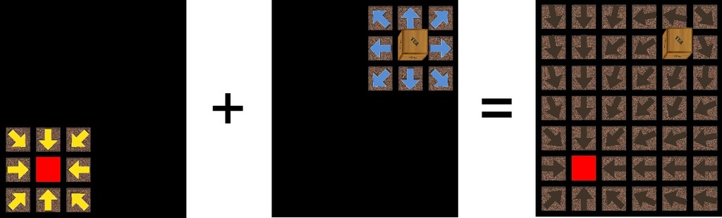
Figure 3. Attractor and Repulsor
Each individual field is calculated by computing the direction toward the attractor and away from repulsors at each point in the room. Once all of the vectors have been calculated, you obtain the complete vector field by adding them up.
For this example, I will have three streams and two compute operators. The list of attractors and repulsors will be used as the input stream. Then, a compute operator will be applied to it to obtain a second stream: the vector field. Finally, a second compute operator will provide another stream: the local minima field.
Why is this a good demonstration of CUDA? When deciding whether an algorithm is a good candidate for parallelization, you should consider the following criteria:
Is the problem compute-intensive?
Can the problem be modeled as a stream process?
Is the code independent of any shared resources?
What sequences of code are independent of any other code?
Can the data be represented as arrays of 32-bit objects?
Are there no optimizations of the sequential algorithm possible?
In my case, the vector field may be large and could take a long time when evaluating the whole field. The path a robot should follow can be modeled easily with streams. There is no access to shared resources, and the computation of each element in the field is independent from all the others.
In terms of computation, robotic engineers usually constrain their algorithms to calculate only the part of the vector field that is needed at a given time, never evaluating the entire vector field. Next, I show you how you can use stream processing for calculating the whole vector field in real time. Let's get started.
Let's develop a sequential version of a vector field calculation algorithm. The input stream is a list of attractors and a list of repulsors, as shown in Figure 2 and without obstacles (Figure 4). The output stream is a matrix called field. The attractors and repulsors are lists of 2-D points that indicate their positions.
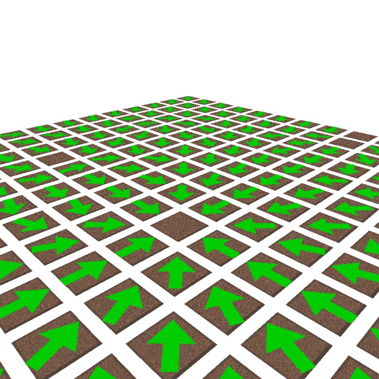
Figure 4. Composing Attractors and Repulsors
A “field” matrix will hold your vector field data structure. Each element field[y][x] will hold a 2-D vector indicating where the robot should move toward when standing at point (x, y). This vector will be the sum of vectors associated with each attractor and repulsor (Figure 5).
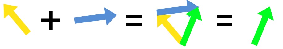
Figure 5. Vector Addition
When processing each attractor, the associated vector will be pointing from the current point (x, y) toward the attractor's position. When processing each repulsor, the associated vector will be pointing away from the repulsor's position. Note that the plus and minus operators are performing vector addition and subtraction. Sequential pseudo-code:
In Parameters: a list of attractors, a list of repulsors
Out Parameters: a zero-initialized vector field

calculate_vector_field_cpu(in attractors, in repulsors, out field):

    for (y = 0 to height):
        for (x = 0 to width):
            for (attractor in attractors):
                vector = attractor - point(x,y)
                field[y][x] = field[y][x] + vector

            for (repulsor in repulsors):
                vector = point(x,y) - repulsor
                if norm(vector) <= 2:
                    field[y][x] = field[y][x] + vector

        return
Okay, so the sequential pseudo-code is ready. Now, let's partition the problem in order to use most of the processing cores on the GPU.
The calculation of each vector field element is independent from the calculation of the other elements. You can leverage this property to parallelize your algorithm. You can calculate each element of the vector field matrix in its own thread, effectively dividing the problem into smaller pieces.
Don't worry about the number of threads. Spawning as many threads as possible when developing CUDA algorithms is encouraged by NVIDIA. It will allow the algorithms to scale across several generations of devices, automatically increasing throughput, as NVIDIA adds more and more processing cores to its video cards.
With this in mind, let's develop a parallel version of our previous algorithm. Parallel pseudo-code:
In Parameters: list of attractors, list of repulsors
Out Parameters: a zero-initialized vector field

calculate_vector_field_gpu(in attractors, in repulsors, out field):

    x = blockIdx.x * BLOCK_SIZE + threadIdx.x
    y = blockIdx.y * BLOCK_SIZE + threadIdx.y

    for (attractor in attractors):
        vector = attractor - point(x,y)
        field[y][x] = field[y][x] + vector

    for (repulsor in repulsors):
        vector = point(x,y) - repulsor
        if norm(vector) <= 2:4444444444
            field[y][x] = field[y][x] + vector

    return
Notice I did away with both external for loops, and the points (x, y) are now calculated using a parallel statement.
The new pseudo-code is implemented as a kernel. A kernel is a function that executes on several GPU cores at the same time. Kernels are launched by a host program controlled from the regular CPU that configures the execution environment and supplies the parameters.
How does each thread know what position of the vector field it has to compute? This is where the blockIdx and threadIdx built-in CUDA variables come into place.
As you look at this code, it may not be obvious how this is a parallel implementation, but it's the blockIdx and threadIdx and the CUDA magic associated with them that makes it parallel. When the function is invoked, it actually is invoked multiple times using multiple threads, each thread calculating one part of the result (see the next section).
When the host code sets up an execution environment, it has to determine how the processing cores will be assigned work. As part of its duties, the host must determine how threads will be arranged logically. CUDA allows developers to arrange their threads in a 1-D, 2-D or 3-D structure. It helps developers express design in a natural manner.
Think about the example algorithm. Let's use the GPU to fill a 2-D matrix with data. It would be very convenient if you somehow could assign each thread a “position” in a two-coordinate system, because each thread could use its assigned coordinates to decide which element to compute.
CUDA provides a mechanism through which developers can specify how they want their threads arranged. The compiler takes care of the rest. This feature is available through what is known as a grid of thread blocks. In this example, the host will use a 2-D grid.
You probably are wondering, why a “grid of thread blocks” instead of a “grid of threads”?
Threads do not exist inside grids by themselves, but rather, they are arranged into thread blocks. Each thread is assigned an identifier within its block. Each block, in turn, is assigned an identifier within the grid. The built-in blockIdx and threadIdx variables help determine the current thread and block identifiers. From within a kernel, these identifiers can be seen simply as a C structure containing the thread's x, y and z coordinates.
Using this mechanism, you can have each thread calculate a global thread ID and calculate the x and y variables in your parallel pseudo-code. The pair (x, y) determines which element of the matrix has to be computed. Because each thread will have different values for (x, y), every point of the matrix could, in theory, be computed at the same time if you have enough threads.
Now, let's apply a second operation that detects local minima on the computed vector field. Local minima are those places where all vectors are converging (Figure 6). Flagging out the local minima will prevent the mobile robot from stopping in one of them with none of the vectors guiding it out.

Figure 6. Three Local Minima the Mobile Robot Should Avoid
Under the stream processing model, operators can be daisy-chained: a second operator consumes the output of a first operator, much like the pipe operator of an operating system. In the example CUDA implementation, you will consume the vector field matrix stored in GPU memory. Sequential local minima detection pseudo-code:
In Parameters: calculated vector field, a decimal threshold
Out Parameters: a boolean matrix called "minima"

detect_local_minima_cpu(in field, in threshold, out minima):

    for (y=0 to h):
        for (x=0 to w):
            minima[y][x] =
                (norm(field[y][x]) < threshold)? true : false

    return
The sequential algorithm takes the vector field as input and fills in a Boolean matrix of the same dimensions with values “true” or “false”, depending on whether the length is below a given threshold. Conversely, the matrix “minima” at position (x, y) indicates whether the norm of the vector located at (x, y) is less than the given threshold. Parallel local minima detection:
In Parameters: the calculated vector field, a decimal threshold
Out Parameters: a boolean matrix called "minima"

detect_local_minima_gpu(in field, in threshold, out minima):
    x = blockIdx.x * BLOCK_SIZE + threadIdx.x
    y = blockIdx.y * BLOCK_SIZE + threadIdx.y
    minima[y][x] = (norm(field[y][x]) < threshold) ? true : false
The output is a field of Boolean values that indicates whether a given point is a local minimum.
At this point, I have implemented four algorithms. You can, of course, download all the source code from our Web site for free and try them out yourself.
So, how does a CUDA algorithm stack up against its CPU equivalent? Next, I compare the parallel versions against their sequential counterparts in order to find out. The hardware used for the benchmark implementation includes:
Intel Core 2 Duo E6320, running at 1.6GHz with 4GB of RAM.
NVIDIA GeForce 8600GT GPU.
Ubuntu Linux 8.10.
CUDA version 2.2.
I implemented all four algorithms in one C++ program that can switch between the CPU and the CUDA versions of the algorithms dynamically. Not only does this make the benchmarking process easier, but it also is a good technique for developing programs that can fall back to the CPU on a computer where CUDA is not supported.
Each of the benchmarks uses different vector field configurations, increasing the size of the field as well as the number of repulsors. The number of attractors always is set to just one. The size of the vector fields are: 16x16, 32x32, 64x64, 128x128 and 256x256. The repulsors are randomly distributed on the field with a ratio of one repulsor per 32 vector field points. Hence, the number of repulsors is 8, 32, 128, 512, 2048 and 8192.
Figure 7 shows the results of the benchmarks. I am using the notation “WxH/R”, where WxH denotes the vector field's dimensions and R the number of repulsors present. The execution time is in milliseconds on a logarithmic scale (so a small difference in graph size is actually a much larger speedup than it appears to be visually).
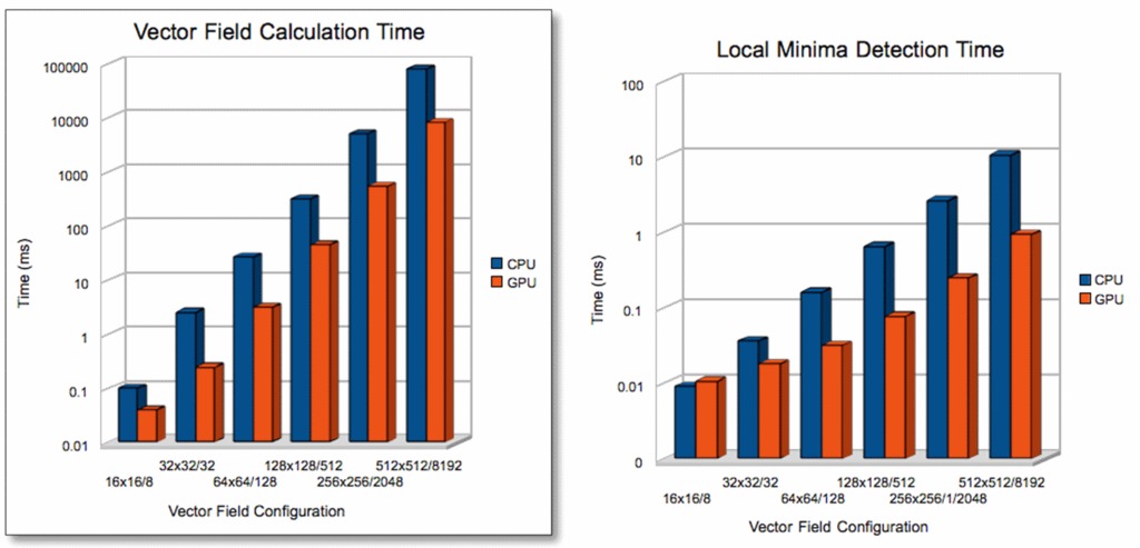
Figure 7. Calculation Times
How much faster is the GPU? The speedup is calculated by dividing the execution time of the sequential algorithm by the execution time of the parallel algorithm (Figure 8).
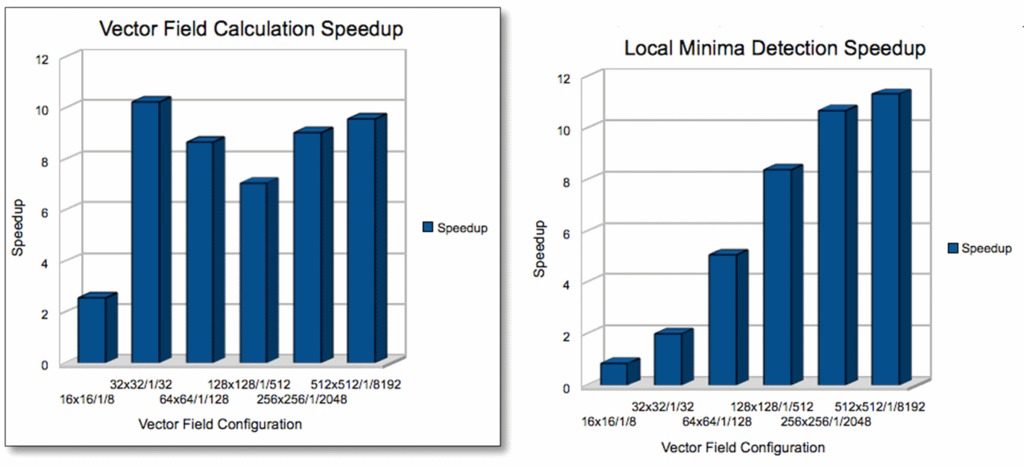
Figure 8. Speedup
Computation times are the closest in the case of a small vector field. However, even in that case, we get a speedup of 2.5 times just by switching to the CUDA implementation of the vector field calculation. The local minima detection becomes interesting to parallelize only with slightly larger data sets that are more compute-intensive than smaller ones.
On average, the speedup is around eight times for our algorithms. In layman's terms, this means if you have a computation that takes one work day to complete, just by switching to CUDA, you can have your results in less than one hour.
This provides significant benefits for computations that require a user to run a computation several times while correcting the parameters each time. Such iterative processes are frequent, for instance, in financial models.
If parallelization of your algorithm is possible, using CUDA will speed up your computations dramatically, allowing you to make the most out of your hardware.
The main challenge consists in deciding how to partition your problem into chunks suitable for parallel execution. As with so many other aspects in parallel programming, this is where experience and—why not—imagination come into play.
Additional techniques offer room for even more improvement. In particular, the on-chip shared memory of each compute node allows further speedup of the computation process.
Resources
Hardware-Accelerated Computation: gpgpu.org
Source Code and Video: www.coroware.com/streamprocessing
Getting Started on CUDA: www.nvidia.com/cuda
ATI-Based Stream SDK: developer.ati.com/gpu/atistreamsdk
OpenCL Official Web Site: www.khronos.org/opencl
Alejandro Segovia is a parallel programming advisor for CoroWare. He is also a contributing partner at RealityFrontier. He works in 3-D graphic development and GPU acceleration. Alejandro was recently a visiting scientist at the University of Delaware where he investigated CUDA from an academic standpoint. His findings were published at the IEEE IPCCC Conference in 2009.