
Introduction to Lisp-Stat
Although I installed Linux on a 80 Meg partition on my Gateway 33Mhz PC over a year ago, I really did not make serious use of Linux for my scientific work, mostly because I lacked disk space. Recently, I bought a new 1-Gig drive and that excuse went away. So I decided to install Lisp-Stat, a program that I use most for my statistical Computing.
Written by Luke Tierney at the University of Minnesota, Lisp-Stat is a powerful, interactive, object-oriented statistical computing environment based on the the Xlisp dialect of Lisp. It runs on under Microsoft Windows, Macs, and Unix based X11 systems almost uniformly. It has good graphical facilities for both static and dynamic graphics along with functions for common statistical computations.
Furthermore, using the foreign function interface, one can call C and Fortran programs from within Lisp-Stat. A byte-code compiler is available to speed up your programs once you have debugged them. Of course, one needn't use Lisp-Stat for statistical computing alone; I routinely use for all kinds of things: as a calculator, for figuring out grades of my students, as an engine for hypertext illustrations as well as matrix manipulations.
In this article, I will introduce you to some of the capabilities of Lisp-Stat. Although I use Lisp in this article, I will not get into the details of Lisp programming unless it impinges on our discussion. If you are new to Lisp, you might want to read article on Scheme by Robert Sanders, Linux Journal, March 1995, as Lisp and Scheme are closely related. Some of the comments I make apply actually to Lisp, but it serves no useful purpose to delineate what is the Lisp and what is the Stat part. You need not know Lisp to use any of the examples or to follow the article. If you get seriously interested in Lisp-Stat you should probably get a copy of Tierney's book titled Lisp-Stat, ISBN 0-471-50916-7, published by John Wiley. Besides being the canonical reference for Lisp-Stat, it provides a quick and practical introduction to Lisp.
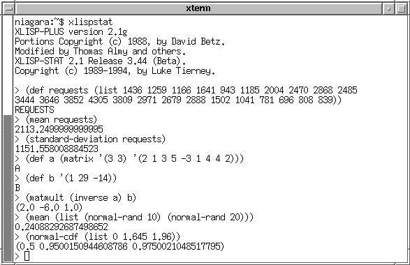
Assuming that you have installed Lisp-Stat successfully, just type xlispstat to invoke the program. To quit the program, just type (exit). Figure 1 shows a simple session. Case does not matter and the > you see in the figure is Lisp-Stat's prompt. The data I have used is the number of requests a WWW server honored during each of the 24 hours in a day. The def macro binds a variable name requests to the list of values.
As the example shows, calculation of summary statistics like the mean and standard deviation are trivial. Since Lisp-Stat is based on Lisp, you have all the power of Lisp for data manipulation. A rich set of data types is available including vectors, sequences, strings, matrices. In figure 1 the variable A is defined to be a 3x3 matrix and B is a list of three numbers. The example solves Ax=b for x by computing A<+>-1<+>b yielding the solution [2, -6, 1]. Note that b is a list while A<+>-1<+> is a matrix, yet the Lisp interpreter takes care of the types and in effect computes the product of a matrix and a vector.
Many of Lisp-Stat's functions operate on sequences which may be lists or vectors and they are vectorized, meaning that these functions can be applied to arguments that are lists and the result is a list of the results of applying the function to each element of the list. Some other functions are vector reducing, meaning that they can be applied to a list of arguments but they return a single number. In figure 1, the function mean is an example of a vector-reducing function; it treated the list of lists as a single long list and returned the mean of the long list. On the other hand, the function normal-cdf is a vectorized function and invoking it on a list of three numbers produces a list of three answers. Of course, if we do wish mean to behave in a vectorized fashion, the statement (mapcar #'mean (list (normal-rand 10) (normal-rand 20))) will do it.
Figure 2: A histogram and a Line Plot
A picture is worth a thousand words, particularly in statistics. Lisp-Stat boasts excellent graphical tools. The graphical system is based on an object-oriented paradigm. Functions that create graphical windows or plots return an object as the result. The returned object is just another data type much like a number or a list and it can be used in appropriate computations.
Commonly used graphical functions are histogram for constructing histograms, plot-points for plotting (x,y) pairs, plot-lines for joining (x,y) pairs by means of lines, plot-function for plotting a function of one variable, spin-function for plotting a function of two variables, and spin-plot for 3-d plots.
All the spin functions provide controls for yawing, pitching and rolling in the graph they create. Figure 2 shows a plot of the number of requests versus each of the 24 hours. The plots were produced using the following lines of code.
(histogram requests)
(def time (iseq 24))
(plot-lines time requests)
(send * :add-points time requests)
(send ** :point-symbol (iseq 24) 'diamond)
Just drawing the lines alone is less than satisfactory since the exact location of the points is lost. So, after constructing the plot, we send a “message” to the plot using the send function asking the object to add-points to the graph resulting in the graph shown. The * in the send function refers to the result of the previous command, i.e., the plot object. The ** refers to the result of the command before the previous one. In the example, I have asked that the plotting symbol be a diamond instead of the default circle. The user has a choice of quite a few plotting symbols.
In each plot there is a menu button that has further useful options. One can select or deselect points with the mouse, highlight certain points, save the plot as a postscript file etc. I will only discuss a single feature, that of linking. Linked plots are a way of sharing information between plots. Consider for example, figure 2, where we have a plot of requests versus time as well as a histogram of requests.
If you enable linking by choosing the Link View item in the menu in each plot, selecting a vertical bar in the histogram by dragging the mouse with the button pressed causes the corresponding points in the line plot to be highlighted. You might have to peer at the figure to see that the point where the highest peak occurs is highlighted since it corresponds to the highlighted histogram bar. Linking is extremely useful in viewing multidimensional data since one can get a better idea of how the same group of points can be projected in different views.
Online documentation for Lisp-Stat is available via the functions help, help* and apropos. For help on the mean function, type (help 'mean). The use of the quote is essential, otherwise the interpreter would assume that mean is a variable and try to evaluate it. However, in many situations, one does not know what the function is named.
For example, is the function that multiples two matrices mat-mult or matrix-multiply? Typing (apropos 'mult) will print a list of all symbols that have the word “mult” in them. This might help you narrow down the search. On the other hand, if you know that the function you are looking for contains the word matrix in it, (help* 'matrix) will return help on all symbols that contain the word matrix. The help facility as it exists now is less than optimal and several people are developing a more elaborate help system.
I usually read the newsgroup sci.stat.math and almost always there is someone out there who wants to know how to calculate an F-probability or how to generate a normal random variable. Lisp-Stat has distribution functions and generators for all of the commonly used distributions. For example (normal-cdf 1.645) will give you the probability to the left of 1.645 which is about 0.95. The statement(def x (normal-rand 100)) will define x to be a list of 100 standard normal variates. Similar functions exist for Students-T, Gamma, Beta, Chi-squared and F distributions as (help* 'cdf) or (help* 'rand) will show.
Lisp-Stat has many functions for input and output. For dealing with files, I've rarely needed to go beyond using the two functions read-data-file and read-data-columns. The statement (read-data-file "foo.dat") returns the whole file contents as one long list, while (read-data-columns "foo.dat") returns a list of columns of the file. One can specify the number of columns in the data file as a second argument to read-data-columns. Otherwise, it guesses the number of columns based on the first line. The function format, which is similar to C's sprintf(), is a versatile function for formatted printing.
Lisp-Stat's graphical system and regression models are implemented using a prototype-based object system. This is different from the class-based object system used by languages like C++ or the approach used by Common Lisp Object System (CLOS). Briefly speaking, there is a root prototype object from which instances of all other objects are created. Objects can have slots to hold information and they respond to messages which are dispatched to the object using the send function. Messages are typically keywords, words that begin with a colon–:add-points in figure 2 is an example.
The code that actually implements the action is called a method for the message. The macros defproto and defmeth make the process of constructing objects and writing methods easier. Lisp-Stat would be less interesting if all it provided were objects for building statistical models. The windowing system provides objects for building user interfaces like menus, dialogs, slider controls etc. So one can construct nice dialogs to go with the computations.
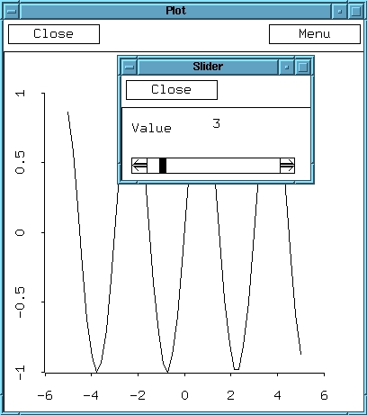
Figure 3 shows an example of dynamic animation using a slider dialog. The function sin2pi x/n is plotted. The slider allows the user to see the plot change as n is changed. The code to perform this is below.
(setf n 1)
(defun f (x) (sin (/ (* 2 pi x) n)))
(def sine-plot (plot-function #'f -5 5))
(defun change-n (x)
  (setf n x)
  (send sine-plot :clear :draw nil)
  (send sine-plot :add-function #'f -5 5))
(sequence-slider-dialog (iseq 1 20) :action #'change-n)
The function sequence-slider-dialog creates a slider. Initially, the global variable n is 1. Every time the user moves the slider-stop using the mouse, the function change-n gets called with the value of n corresponding to the slider-stop. In our example, n can be any integer from 1 to 20. The function change-n sets the value of n and redraws the plot.
In order to keep the discussion tolerable, I chose a simple example that is probably not too useful. For serious programming, one needs to know about the built-in prototypes and functions of Lisp-Stat discussed in Tierney's book. I shall introduce what I need as I go along.
We will create an object that accepts a list of (x,y) values and draws a plot with the least-squares line superimposed on it. We will also require that the equation of the least-squares line be displayed in the plot. We begin by defining a new prototype. It is only natural that our prototype be a descendent of the built-in prototype scatterplot-proto which “knows” all about drawing 2D plots.
(defproto least-squares-plot-proto '(intercept slope) ()
          scatterplot-proto)
Notice that our prototype has two slots for holding the intercept and the slope of the least squares line. We will need to access the values in these slots later, so it is best to define two simple methods using the defmeth macro that return the slot values.
(defmeth least-squares-plot-proto :slope ()
 "Returns the slope of the least squares line."
  (slot-value 'slope))
(defmeth least-squares-plot-proto :intercept ()
 "Returns the intercept of the least squares line."
  (slot-value 'intercept))
We have provided a documentation string for the methods; the documentation can be retrieved by means of a command such as (send least-squares-plot-proto :help :slope).
In order to use our prototype, we must define a :isnew method that initializes an instance of the prototype. Our :isnew method must calculate the least-squares line and store the slope and intercept. It should exploit its lineage as a descendant of scatterplot-proto by invoking the inherited methods to do the plotting tasks. Some space must be created in the margin to display the equation for the least-squares line.
Finally, the x,y points must be plotted, the axes labeled, and the window redrawn to reflect the changes. Here is the method.
(defmeth least-squares-plot-proto :isnew (x y &key (title "LS Plot"))
  (let* ((m (regression-model x y :print nil))
         (beta (send m :coef-estimates)))
    (setf (slot-value 'intercept) (select beta 0))
    (setf (slot-value 'slope) (select beta 1)))
  (call-next-method 2 :title title)
  (send self :margin 0 (+ (send self :text-ascent)
                          (send self :text-descent)) 0 0)
  (send self :add-points x y)
  (send self :variable-label 0 "X")
  (send self :variable-label 1 "Y")
  (send self :redraw))
We have used the regression-model function to compute the least-squares line. The call-next-method function calls the :isnew inherited method of scatterplot-proto–this is what actually creates a plot-window. The argument 2 just refers to the number of variables that will be plotted. At this point, the plot-window is actually blank. Using information about the font in use, a margin area is created. Then the points are plotted. In the body of a method the variable self is bound to the object receiving the message. The method concludes by giving some meaningful names to the variables and redrawing the window.
All the above code will do is plot the points. How can we ensure that least-squares line and its equation are also displayed? We use the fact that any window is actually drawn using a :redraw message. By writing a new :redraw message, we can ensure the results we want. In actuality, the :redraw message itself is executed via three other messages :redraw-background, :redraw-content and :redraw-overlays. We really only need to write a :redraw-content method since only the content of the plot is affected. So here we go.
(defmeth least-squares-plot-proto :redraw-content ()
  (call-next-method)  ; Let the scatterplot do its things.
  (send self :adjust-to-data :draw nil) ; make sure scale is ok.
  (let* ((limits (send self :range 0))
         (intercept (send self :intercept))
         (slope (send self :slope))
         (info-str (format nil "y = ~5,3f + ~5,3f x" intercept slope)))
    (send self :draw-string info-str
          10 (+ (send self :text-ascent) (send self :text-descent)))
          ; Display the equation in the margin.
    (send self :add-function ; Draw the LS line.
          #'(lambda (x) (+ intercept (* slope x)))
          (car limits)
          (cadr limits) :draw nil)))
Notice that the keyword argument :draw is nil to avoid infinite loops in the redrawing process. If :draw is not nil, the :redraw method gets invoked again. The line is actually drawn using the :add-function method of scatterplot-proto. We need not worry about drawing the points since that is the responsibility of scatterplot-proto once we have added the points in the :isnew method.
Figure 4 shows the results of using this code with the following program.
(def x (normal-rand 20))
(def y (+ 5 (* 2 x) (normal-rand 20)))
(def m (send least-squares-plot-proto :new x y))
Compiling a Lisp-Stat program is straightforward. The statement (compile-file "foo") in Lisp-Stat will compile the file foo into foo.fsl. When you load the file foo later, the compiled file is loaded if it exists and is newer than the uncompiled file. Debugging can be accomplished via the debug, baktrace and trace functions. A stepper is also available to step through lines of code.
There are many interesting dynamic animations can be constructed in Lisp-Stat. This article has only scratched the surface. Lisp-Stat continues to evolve and Xlisp itself continues to move closer and closer to Common Lisp due to the efforts of many, particularly Tom Almy and Luke Tierney. The available body of applications and software for Lisp-Stat is also growing; see the sidebar “Getting Lisp-Stat” for more information.
Balasubramanian Narasimhan teaches Statistics at Penn State Erie, The Behrend College. His interests include classical western music, Seminole football and the history of India. He may be reached at naras@euler.bd.psu.edu
Lisp-Stat is freely available on the net. The primary distribution site is ftp.stat.umn.edu. Look under pub/xlispstat for xlispstat-3-44.tar.gz. The file is about 1.2 Megabytes, which means that it fits nicely on a 3.5-inch disk. It compiles out of the box on Linux, but to use the foreign-function interface, you must first install the GNU dld library, available from tsx-11.mit.edu under pub/linux/binaries/libs as dld-3.2.5.bin.tar.gz. For those who don't want the adventure of building from scratch, you can obtain a binary from euler.bd.psu.edu under pub/lj/xlispstat. Follow the instructions in the README file. The file xlispstat-3.44-bin.tar.gz is the whole binary.
There is a mailing list for Xlisp-Stat users. To join the mailing list send a message with your e-mail address saying that you want to subscribe to stat-lisp-news-request@stat.umn.edu.
The Usenet newsgroup comp.lang.lisp.x is devoted to XLisp, however it is a low-volume newsgroup averaging 2-3 articles a day.
The site ftp.stat.ucla.edu has a good amount of Lisp and Lisp-Stat related stuff. For a look at some hypertext applications, look at the sites euler.bd.psu.edu and www.stat.ucla.edu.
